Distinguish between different data types and structures in R
Import data from CSV and other file formats
Clean datasets by handling missing values and inconsistencies
Transform data using dplyr verbs (filter, select, mutate, summarize)
Perform initial exploratory data analysis to understand dataset properties
This chapter covers the fundamental concepts of working with data in R. You’ll learn how to import, clean, and prepare data for analysis, which are essential skills for any data analysis project across all natural science disciplines.
2.2 Understanding Data Structures
Before diving into data analysis, it’s important to understand the basic data structures in R:
2.2.1 Data Types
R has several basic data types:
Numeric: Decimal values (e.g., measurements of temperature, pH, concentration, or distance)
Integer: Whole numbers (e.g., counts of organisms, samples, or observations)
Character: Text strings (e.g., species names, site descriptions, or treatment labels)
Logical: TRUE/FALSE values (e.g., presence/absence data or condition met/not met)
Factor: Categorical variables with levels (e.g., experimental treatments, taxonomic classifications, or soil types)
Date/Time: Temporal data (e.g., sampling dates, observation times, or seasonal markers)
Code
# Examples of different data typesnumeric_example<-25.4# Temperature in Celsiuscharacter_example<-"Adelie"# Penguin specieslogical_example<-TRUE# Presence/absence datafactor_example<-factor(c("Control", "Treatment", "Control"), levels =c("Control", "Treatment"))date_example<-as.Date("2020-07-15")# Sampling date# Print examplesprint(numeric_example)#> [1] 25.4print(character_example)#> [1] "Adelie"print(logical_example)#> [1] TRUEprint(factor_example)#> [1] Control Treatment Control #> Levels: Control Treatmentprint(date_example)#> [1] "2020-07-15"
Code Explanation
This code demonstrates the fundamental data types in R:
Numeric Data:
Created a decimal value representing temperature in Celsius
Common for environmental measurements and continuous data
Character Data:
Created a text string for a penguin species name
Used for categorical variables like species names or site descriptions
Logical Data:
Created a TRUE value representing presence/absence
Used for binary data or conditions in analyses
Factor Data:
Created an ordered categorical variable with two levels
Explicitly defined factor levels (“Control” and “Treatment”)
Essential for statistical analyses and proper plotting order
Date Data:
Created a date object using the as.Date() function
Used for temporal data in ecological studies
Results Interpretation
The output shows how R stores and displays different data types:
Numeric Data:
Displayed as 25.4 without type indication
R treats this as a continuous numeric value for calculations
Character Data:
Displayed as “Adelie” with quotation marks indicating text
Cannot be used for numerical operations
Logical Data:
Displayed as TRUE (without quotation marks)
Can be used in conditional operations and converts to 1 (TRUE) or 0 (FALSE) in calculations
Factor Data:
Displayed with levels information: Control, Treatment, Control
Internally stored as integers with labels
Order of levels is preserved as specified
Date Data:
Displayed in standardized YYYY-MM-DD format
Allows for time-based calculations and comparisons
PROFESSIONAL TIP: Data Management Best Practices
Proper data management is critical for reproducible research in natural sciences:
Document metadata: Always maintain detailed records about data collection methods, units, and variable definitions
Use consistent naming conventions: Create clear, consistent file and variable names (e.g., site_01_temp_2023.csv instead of data1.csv)
Preserve raw data: Never modify your original data files; always work with copies for cleaning and analysis
Version control: Use Git or similar tools to track changes to your data processing scripts
Implement quality control: Create automated checks for impossible values, outliers, and inconsistencies
Plan for missing data: Develop a consistent strategy for handling missing values before analysis begins
Create tidy data: Structure data with one observation per row and one variable per column
Use open formats: Store data in non-proprietary formats (CSV, TSV) for long-term accessibility
Back up regularly: Maintain multiple copies of your data in different physical locations
Consider data repositories: Share your data through repositories like Dryad, Zenodo, or discipline-specific databases
2.2.2 Data Structures in R
R has several data structures for organizing information:
Code
# Load real datasetslibrary(readr)penguins<-read_csv("../data/environmental/climate_data.csv")crops<-read_csv("../data/agriculture/crop_yields.csv")# Vector example - penguin bill lengthsbill_lengths<-na.omit(penguins$bill_length_mm[1:10])print(bill_lengths)#> [1] 39.1 39.5 40.3 36.7 39.3 38.9 39.2 34.1 42.0#> attr(,"na.action")#> [1] 4#> attr(,"class")#> [1] "omit"# Matrix example - create a matrix from penguin measurementspenguin_matrix<-as.matrix(penguins[1:5, 3:6])print(penguin_matrix)#> bill_length_mm bill_depth_mm flipper_length_mm body_mass_g#> [1,] 39.1 18.7 181 3750#> [2,] 39.5 17.4 186 3800#> [3,] 40.3 18.0 195 3250#> [4,] NA NA NA NA#> [5,] 36.7 19.3 193 3450# Data frame example - first few rows of penguin datapenguin_data<-penguins[1:5, ]print(penguin_data)#> # A tibble: 5 × 8#> species island bill_length_mm bill_depth_mm flipper_length_mm body_mass_g#> <chr> <chr> <dbl> <dbl> <dbl> <dbl>#> 1 Adelie Torgersen 39.1 18.7 181 3750#> 2 Adelie Torgersen 39.5 17.4 186 3800#> 3 Adelie Torgersen 40.3 18 195 3250#> 4 Adelie Torgersen NA NA NA NA#> 5 Adelie Torgersen 36.7 19.3 193 3450#> # ℹ 2 more variables: sex <chr>, year <dbl># List example - store different aspects of the datasetpenguin_summary<-list( species =unique(penguins$species), avg_bill_length =mean(penguins$bill_length_mm, na.rm =TRUE), sample_size =nrow(penguins), years =unique(penguins$year))print(penguin_summary)#> $species#> [1] "Adelie" "Gentoo" "Chinstrap"#> #> $avg_bill_length#> [1] 43.92193#> #> $sample_size#> [1] 344#> #> $years#> [1] 2007 2008 2009
Code Explanation
This code demonstrates the main data structures in R using real ecological datasets:
Data Loading:
Uses readr::read_csv() to import real datasets on penguins and crop yields
Creating new variables from existing ones is a common data preparation task:
Code
# Create new variables in the penguins datasetpenguins_derived<-penguins%>%filter(!is.na(bill_length_mm)&!is.na(bill_depth_mm))%>%mutate( bill_ratio =bill_length_mm/bill_depth_mm, size_category =case_when(body_mass_g<3500~"Small",body_mass_g<4500~"Medium",TRUE~"Large"))# View the new variableshead(select(penguins_derived, species, bill_length_mm, bill_depth_mm,bill_ratio, body_mass_g, size_category), 5)#> # A tibble: 5 × 6#> species bill_length_mm bill_depth_mm bill_ratio body_mass_g size_category#> <chr> <dbl> <dbl> <dbl> <dbl> <chr> #> 1 Adelie 39.1 18.7 2.09 3750 Medium #> 2 Adelie 39.5 17.4 2.27 3800 Medium #> 3 Adelie 40.3 18 2.24 3250 Small #> 4 Adelie 36.7 19.3 1.90 3450 Small #> 5 Adelie 39.3 20.6 1.91 3650 Medium
2.5 Data Manipulation with dplyr
The dplyr package provides a powerful grammar for data manipulation:
Code
library(dplyr)# Filter rows - only Adelie penguinsadelie_penguins<-penguins%>%filter(species=="Adelie")head(adelie_penguins, 3)#> # A tibble: 3 × 8#> species island bill_length_mm bill_depth_mm flipper_length_mm body_mass_g#> <chr> <chr> <dbl> <dbl> <dbl> <dbl>#> 1 Adelie Torgersen 39.1 18.7 181 3750#> 2 Adelie Torgersen 39.5 17.4 186 3800#> 3 Adelie Torgersen 40.3 18 195 3250#> # ℹ 2 more variables: sex <chr>, year <dbl># Select columns - focus on measurementspenguin_measurements<-penguins%>%select(species, island, bill_length_mm, bill_depth_mm, flipper_length_mm, body_mass_g)head(penguin_measurements, 3)#> # A tibble: 3 × 6#> species island bill_length_mm bill_depth_mm flipper_length_mm body_mass_g#> <chr> <chr> <dbl> <dbl> <dbl> <dbl>#> 1 Adelie Torgersen 39.1 18.7 181 3750#> 2 Adelie Torgersen 39.5 17.4 186 3800#> 3 Adelie Torgersen 40.3 18 195 3250# Create new variablespenguins_analyzed<-penguins%>%mutate( bill_ratio =bill_length_mm/bill_depth_mm, body_mass_kg =body_mass_g/1000)head(select(penguins_analyzed, species, bill_ratio, body_mass_kg), 3)#> # A tibble: 3 × 3#> species bill_ratio body_mass_kg#> <chr> <dbl> <dbl>#> 1 Adelie 2.09 3.75#> 2 Adelie 2.27 3.8 #> 3 Adelie 2.24 3.25# Summarize data by speciespenguin_summary<-penguins%>%group_by(species)%>%summarize( count =n(), avg_bill_length =mean(bill_length_mm, na.rm =TRUE), avg_bill_depth =mean(bill_depth_mm, na.rm =TRUE), avg_body_mass =mean(body_mass_g, na.rm =TRUE))%>%arrange(desc(avg_body_mass))print(penguin_summary)#> # A tibble: 3 × 5#> species count avg_bill_length avg_bill_depth avg_body_mass#> <chr> <int> <dbl> <dbl> <dbl>#> 1 Gentoo 124 47.5 15.0 5076.#> 2 Chinstrap 68 48.8 18.4 3733.#> 3 Adelie 152 38.8 18.3 3701.# Analyze crop yields datacrop_summary<-crops%>%filter(!is.na(`Wheat (tonnes per hectare)`))%>%group_by(Entity)%>%summarize( years_recorded =n(), avg_wheat_yield =mean(`Wheat (tonnes per hectare)`, na.rm =TRUE), max_wheat_yield =max(`Wheat (tonnes per hectare)`, na.rm =TRUE))%>%arrange(desc(avg_wheat_yield))%>%head(10)# Top 10 countries by average wheat yieldprint(crop_summary)#> # A tibble: 10 × 4#> Entity years_recorded avg_wheat_yield max_wheat_yield#> <chr> <int> <dbl> <dbl>#> 1 Belgium 19 8.54 10.0 #> 2 Netherlands 58 7.03 9.29#> 3 Ireland 58 6.83 10.7 #> 4 United Kingdom 58 6.37 8.98#> 5 Denmark 58 6.18 8.24#> 6 Luxembourg 19 5.98 6.82#> 7 Germany 58 5.89 8.63#> 8 Europe, Western 58 5.72 7.88#> 9 France 58 5.65 7.80#> 10 Northern Europe 58 5.59 7.21
2.6 Exploratory Data Analysis
Before diving into formal statistical tests, it’s essential to explore your data:
Code
# Basic summary statisticssummary(penguins$bill_length_mm)#> Min. 1st Qu. Median Mean 3rd Qu. Max. NA's #> 32.10 39.23 44.45 43.92 48.50 59.60 2summary(penguins$flipper_length_mm)#> Min. 1st Qu. Median Mean 3rd Qu. Max. NA's #> 172.0 190.0 197.0 200.9 213.0 231.0 2summary(penguins$body_mass_g)#> Min. 1st Qu. Median Mean 3rd Qu. Max. NA's #> 2700 3550 4050 4202 4750 6300 2# Correlation between variablescor_matrix<-cor(penguins%>%select(bill_length_mm, bill_depth_mm, flipper_length_mm, body_mass_g), use ="complete.obs")print(cor_matrix)#> bill_length_mm bill_depth_mm flipper_length_mm body_mass_g#> bill_length_mm 1.0000000 -0.2350529 0.6561813 0.5951098#> bill_depth_mm -0.2350529 1.0000000 -0.5838512 -0.4719156#> flipper_length_mm 0.6561813 -0.5838512 1.0000000 0.8712018#> body_mass_g 0.5951098 -0.4719156 0.8712018 1.0000000# Basic visualization - histogram of bill lengthslibrary(ggplot2)ggplot(penguins, aes(x =bill_length_mm))+geom_histogram(binwidth =1, fill ="skyblue", color ="black")+labs(title ="Distribution of Penguin Bill Lengths", x ="Bill Length (mm)", y ="Frequency")+theme_minimal()# Boxplot of body mass by speciesggplot(penguins, aes(x =species, y =body_mass_g, fill =species))+geom_boxplot()+labs(title ="Body Mass by Penguin Species", x ="Species", y ="Body Mass (g)")+theme_minimal()+theme(legend.position ="none")# Scatterplot of bill length vs. flipper lengthggplot(penguins, aes(x =flipper_length_mm, y =bill_length_mm, color =species))+geom_point(alpha =0.7)+labs(title ="Bill Length vs. Flipper Length", x ="Flipper Length (mm)", y ="Bill Length (mm)")+theme_minimal()
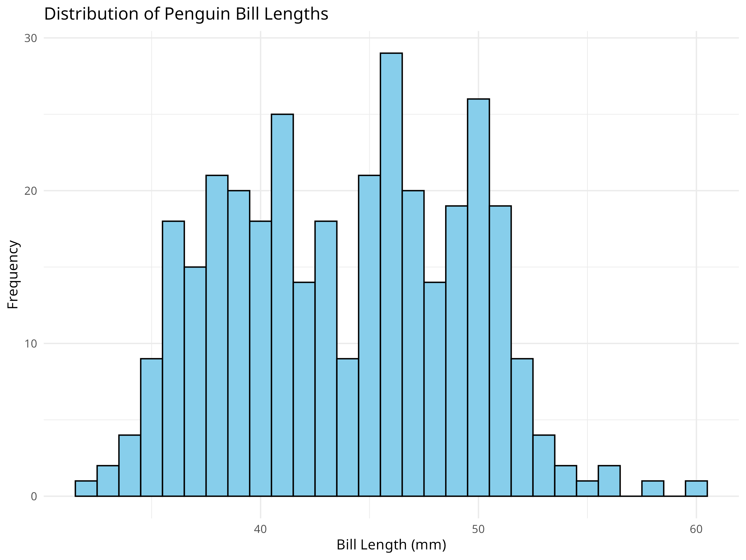
Figure 2.1: Distribution of penguin bill lengths
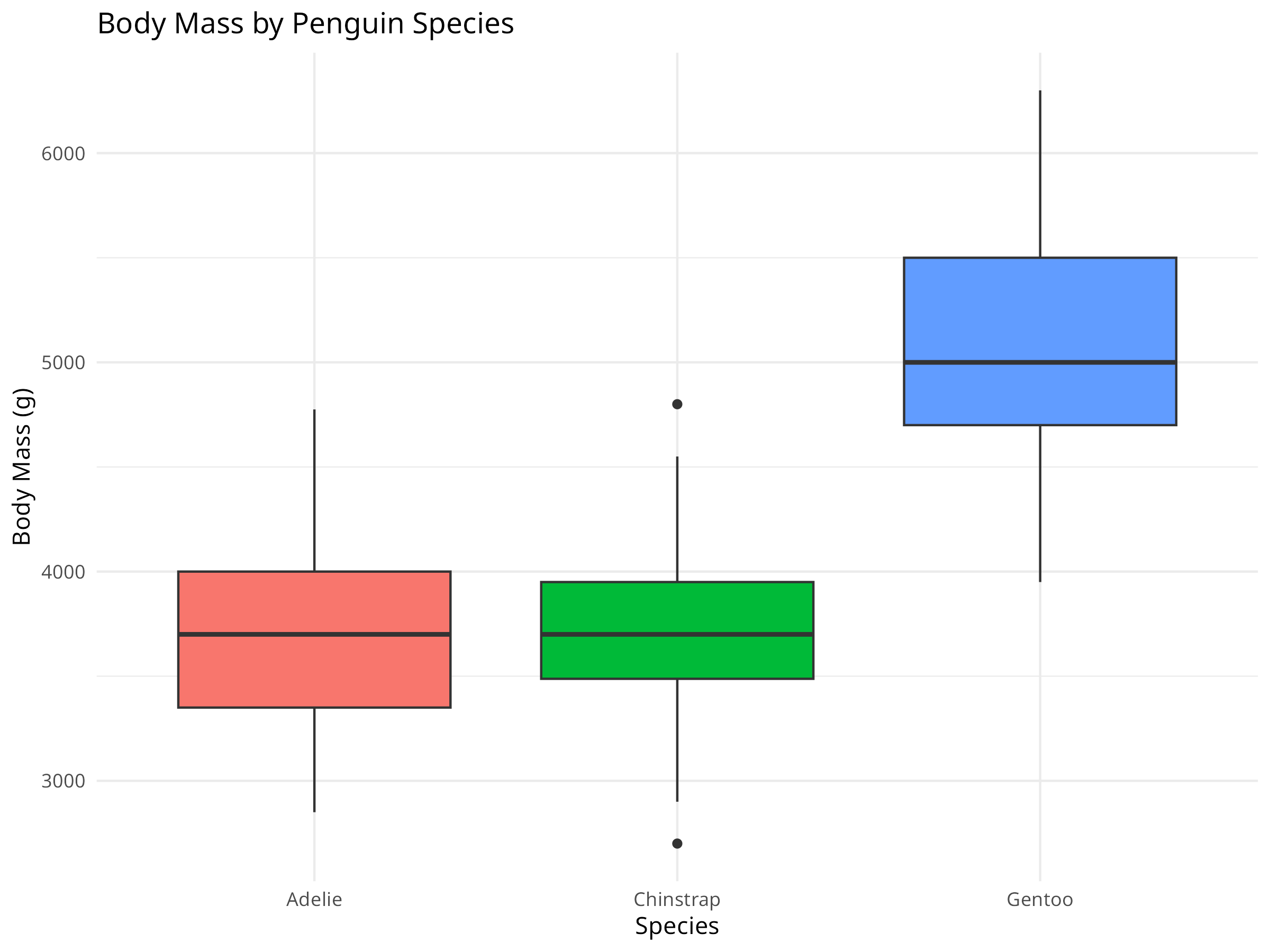
Figure 2.2: Body mass distribution by penguin species
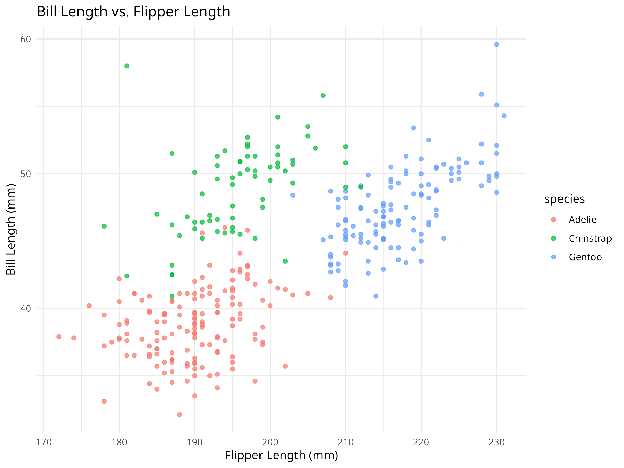
Figure 2.3: Relationship between bill length and flipper length
Code Explanation
This code demonstrates several key data analysis and visualization techniques:
Summary Statistics:
summary() provides descriptive statistics for each variable
Includes min, max, quartiles, mean, and missing values
Correlation Analysis:
cor() calculates correlation coefficients between variables
Some variables have missing values that need attention
Species Differences:
The boxplot shows clear species-specific body mass patterns
Some species show more variation than others
Potential outliers are visible in the body mass data
Morphological Relationships:
The scatterplot reveals correlations between bill and flipper lengths
Species clusters are visible in the morphological space
Some species show distinct morphological patterns
PROFESSIONAL TIP: Exploratory Data Analysis Best Practices
When conducting exploratory data analysis:
Data Quality:
Always check for missing values first
Look for outliers and potential errors
Verify data types and ranges
Visualization Strategy:
Start with simple plots (histograms, boxplots)
Progress to more complex visualizations
Use appropriate plot types for your data
Consider colorblind-friendly palettes
Statistical Summary:
Calculate both descriptive and inferential statistics
Consider the distribution of your data
Look for patterns and relationships
Document any unusual findings
2.7 Summary
In this chapter, we’ve covered the basics of working with data in R:
Understanding different data types and structures
Importing data from various file formats
Cleaning and preparing data for analysis
Creating new variables
Using dplyr for powerful data manipulation
Conducting initial exploratory data analysis
These skills form the foundation for all the analyses we’ll perform in the subsequent chapters. By mastering these basics, you’ll be well-prepared to tackle more complex analytical challenges in various scientific fields.
2.8 Exercises
Load the Palmer Penguins dataset (../data/environmental/climate_data.csv) and create a summary of the number of penguins by species and island.
Calculate the mean and standard deviation of bill length, bill depth, and body mass for each penguin species.
Create a new variable that represents the ratio of flipper length to body mass. Interpret what this ratio might represent biologically.
Create a visualization that shows the relationship between bill length and bill depth, colored by species.
Load the crop yields dataset (../data/agriculture/crop_yields.csv) and analyze trends in wheat yields over time for a country of your choice.
Compare the distributions of body mass between male and female penguins using appropriate visualizations.
Source Code
---prefer-html: true---# Data Basics## Introduction::: {.callout-note}## Learning ObjectivesBy the end of this chapter, you will be able to:1. Distinguish between different data types and structures in R2. Import data from CSV and other file formats3. Clean datasets by handling missing values and inconsistencies4. Transform data using `dplyr` verbs (filter, select, mutate, summarize)5. Perform initial exploratory data analysis to understand dataset properties:::This chapter covers the fundamental concepts of working with data in R. You'll learn how to import, clean, and prepare data for analysis, which are essential skills for any data analysis project across all natural science disciplines.## Understanding Data StructuresBefore diving into data analysis, it's important to understand the basic data structures in R:### Data TypesR has several basic data types:- **Numeric**: Decimal values (e.g., measurements of temperature, pH, concentration, or distance)- **Integer**: Whole numbers (e.g., counts of organisms, samples, or observations)- **Character**: Text strings (e.g., species names, site descriptions, or treatment labels)- **Logical**: TRUE/FALSE values (e.g., presence/absence data or condition met/not met)- **Factor**: Categorical variables with levels (e.g., experimental treatments, taxonomic classifications, or soil types)- **Date/Time**: Temporal data (e.g., sampling dates, observation times, or seasonal markers)```{r}#| label: data-types-examples# Examples of different data typesnumeric_example <-25.4# Temperature in Celsiuscharacter_example <-"Adelie"# Penguin specieslogical_example <-TRUE# Presence/absence datafactor_example <-factor(c("Control", "Treatment", "Control"),levels =c("Control", "Treatment"))date_example <-as.Date("2020-07-15") # Sampling date# Print examplesprint(numeric_example)print(character_example)print(logical_example)print(factor_example)print(date_example)```::: {.callout-note}## Code ExplanationThis code demonstrates the fundamental data types in R:1. **Numeric Data**: - Created a decimal value representing temperature in Celsius - Common for environmental measurements and continuous data2. **Character Data**: - Created a text string for a penguin species name - Used for categorical variables like species names or site descriptions3. **Logical Data**: - Created a TRUE value representing presence/absence - Used for binary data or conditions in analyses4. **Factor Data**: - Created an ordered categorical variable with two levels - Explicitly defined factor levels ("Control" and "Treatment") - Essential for statistical analyses and proper plotting order5. **Date Data**: - Created a date object using the `as.Date()` function - Used for temporal data in ecological studies:::::: {.callout-important}## Results InterpretationThe output shows how R stores and displays different data types:1. **Numeric Data**: - Displayed as 25.4 without type indication - R treats this as a continuous numeric value for calculations2. **Character Data**: - Displayed as "Adelie" with quotation marks indicating text - Cannot be used for numerical operations3. **Logical Data**: - Displayed as TRUE (without quotation marks) - Can be used in conditional operations and converts to 1 (TRUE) or 0 (FALSE) in calculations4. **Factor Data**: - Displayed with levels information: Control, Treatment, Control - Internally stored as integers with labels - Order of levels is preserved as specified5. **Date Data**: - Displayed in standardized YYYY-MM-DD format - Allows for time-based calculations and comparisons:::::: {.callout-tip}## PROFESSIONAL TIP: Data Management Best PracticesProper data management is critical for reproducible research in natural sciences:- **Document metadata**: Always maintain detailed records about data collection methods, units, and variable definitions- **Use consistent naming conventions**: Create clear, consistent file and variable names (e.g., `site_01_temp_2023.csv` instead of `data1.csv`)- **Preserve raw data**: Never modify your original data files; always work with copies for cleaning and analysis- **Version control**: Use Git or similar tools to track changes to your data processing scripts- **Implement quality control**: Create automated checks for impossible values, outliers, and inconsistencies- **Plan for missing data**: Develop a consistent strategy for handling missing values before analysis begins- **Create tidy data**: Structure data with one observation per row and one variable per column- **Use open formats**: Store data in non-proprietary formats (CSV, TSV) for long-term accessibility- **Back up regularly**: Maintain multiple copies of your data in different physical locations- **Consider data repositories**: Share your data through repositories like Dryad, Zenodo, or discipline-specific databases:::### Data Structures in RR has several data structures for organizing information:```{r}#| label: data-structures# Load real datasetslibrary(readr)penguins <-read_csv("../data/environmental/climate_data.csv")crops <-read_csv("../data/agriculture/crop_yields.csv")# Vector example - penguin bill lengthsbill_lengths <-na.omit(penguins$bill_length_mm[1:10])print(bill_lengths)# Matrix example - create a matrix from penguin measurementspenguin_matrix <-as.matrix(penguins[1:5, 3:6])print(penguin_matrix)# Data frame example - first few rows of penguin datapenguin_data <- penguins[1:5, ]print(penguin_data)# List example - store different aspects of the datasetpenguin_summary <-list(species =unique(penguins$species),avg_bill_length =mean(penguins$bill_length_mm, na.rm =TRUE),sample_size =nrow(penguins),years =unique(penguins$year))print(penguin_summary)```::: {.callout-note}## Code ExplanationThis code demonstrates the main data structures in R using real ecological datasets:1. **Data Loading**: - Uses `readr::read_csv()` to import real datasets on penguins and crop yields - Loads data with proper data types and handling2. **Vector Creation**: - Creates a numeric vector of bill lengths - Uses `na.omit()` to remove missing values - Subsets only the first 10 values with `[1:10]`3. **Matrix Construction**: - Creates a numeric matrix from penguin measurements - Uses `as.matrix()` to convert data frame columns to matrix - Selects rows 1-5 and columns 3-6 using indexing4. **Data Frame Handling**: - Demonstrates a data frame (the most common data structure) - Shows how to subset rows while keeping all columns5. **List Creation**: - Creates a list to store heterogeneous data elements - Contains different data types: character vector, numeric value, and integer - Demonstrates how lists can store complex, nested information:::::: {.callout-important}## Results InterpretationThe output reveals the structure and properties of different R data types:1. **Vector Output**: - Shows a one-dimensional array of bill length measurements - All elements are of the same type (numeric) - Suitable for storing a single variable's values2. **Matrix Output**: - Displays a two-dimensional array of measurements - All values must be of the same type (converted to numeric) - Row and column indices are shown - Efficient for mathematical operations but less flexible than data frames3. **Data Frame Output**: - Shows a tabular structure with different variable types - Preserves column names and data types - The foundation of most data analysis in R - Each column can have a different data type4. **List Output**: - Displays a collection of disparate elements - Shows the flexibility of lists for storing mixed data - Demonstrates named elements for easy access - Ideal for storing complex results and heterogeneous data:::## Importing Data### Reading Data FilesR provides several functions for importing data from different file formats:```{r}#| label: import-data# CSV files - Palmer Penguins datasetpenguins_csv <-read.csv("../data/environmental/climate_data.csv")head(penguins_csv, 3)# Using the tidyverse approach for better handlinglibrary(tidyverse)penguins_tidy <- readr::read_csv("../data/environmental/climate_data.csv")head(penguins_tidy, 3)# Crop yields datasetcrops_csv <-read.csv("../data/agriculture/crop_yields.csv")head(crops_csv, 3)```::: {.callout-note}## Code ExplanationThis code demonstrates different methods for importing data in R:1. **Base R Import**: - Uses `read.csv()` from base R to import the penguin dataset - Simple approach that works without additional packages - Generally slower for large datasets and less flexible with column types2. **Tidyverse Import**: - Uses `readr::read_csv()` from the tidyverse ecosystem - More efficient for large datasets and better type inference - Maintains consistent column types and handles problematic values better3. **Data Preview**: - Uses `head()` with argument `3` to display just the first three rows - Allows quick inspection of data structure without overwhelming output - Essential first step to verify successful import and correct structure4. **Multiple Datasets**: - Demonstrates importing different datasets (penguins and crop yields) - Shows the same approach works across various data sources:::::: {.callout-important}## Results InterpretationThe output reveals differences between import methods and gives insight into the datasets:1. **Data Structure Visibility**: - Both datasets show proper column names and values - The tidyverse import (readr) provides cleaner output with column types - Types are indicated (<dbl> for numeric, <chr> for character, etc.)2. **Import Method Comparison**: - Base R (`read.csv()`) and tidyverse (`read_csv()`) produce similar results - Tidyverse version provides more metadata about column types - Both successfully imported the data with proper structure3. **Data Content Preview**: - Penguin data contains morphological measurements and categorical variables - Crop yield data includes countries, years, and production statistics - Both datasets appear properly formatted for analysis:::### Exploring Real-World DatasetsLet's explore some of the real-world datasets we have available:```{r}#| label: explore-datasets# Palmer Penguins datasetpenguins <-read_csv("../data/environmental/climate_data.csv")glimpse(penguins)# Basic summary statisticssummary(penguins$bill_length_mm)summary(penguins$flipper_length_mm)# Crop yields datasetcrops <-read_csv("../data/agriculture/crop_yields.csv")glimpse(crops)```## Data Cleaning and Preparation### Handling Missing ValuesMissing values are common in scientific datasets and need to be addressed before analysis:```{r}#| label: handle-missing-values# Check for missing values in the penguins datasetsum(is.na(penguins))colSums(is.na(penguins))# Create a complete cases datasetpenguins_complete <-na.omit(penguins)print(paste("Original dataset rows:", nrow(penguins)))print(paste("Complete cases rows:", nrow(penguins_complete)))# Replace missing values with the mean for numeric columnspenguins_imputed <- penguinspenguins_imputed$bill_length_mm[is.na(penguins_imputed$bill_length_mm)] <-mean(penguins_imputed$bill_length_mm, na.rm =TRUE)penguins_imputed$bill_depth_mm[is.na(penguins_imputed$bill_depth_mm)] <-mean(penguins_imputed$bill_depth_mm, na.rm =TRUE)# Check if missing values were replacedsum(is.na(penguins_imputed$bill_length_mm))```::: {.callout-note}## Code ExplanationThis code demonstrates essential techniques for handling missing values in ecological data:1. **Missing Value Detection**: - Uses `is.na()` to identify missing values in the dataset - `sum(is.na())` counts the total number of missing values - `colSums(is.na())` reports missing values per column - Critical first step in data cleaning2. **Complete Case Analysis**: - Uses `na.omit()` to remove rows with any missing values - Creates a new dataset (`penguins_complete`) with only complete rows - Compares the row count before and after removal - Simple but can lead to significant data loss3. **Mean Imputation**: - Creates a copy of the original dataset (`penguins_imputed`) - Replaces missing values with column means - Uses logical indexing with `is.na()` to target only missing values - Calculates means with `na.rm = TRUE` to ignore missing values - Verifies imputation success with another missing value check:::::: {.callout-important}## Results InterpretationThe output reveals the extent and impact of missing data:1. **Missing Data Quantity**: - The total number of missing values in the dataset - The distribution of missing values across columns - Some columns (like bill measurements) have more missing values than others2. **Data Loss Impact**: - The original dataset has more rows than the complete cases dataset - The difference represents the number of incomplete observations - In ecological studies, this data loss can introduce bias if missingness isn't random3. **Imputation Effectiveness**: - After imputation, specific columns no longer contain missing values - The final check (showing 0) confirms successful imputation - This approach preserves sample size but may reduce variability:::::: {.callout-tip}## PROFESSIONAL TIP: Handling Missing Values in Ecological DataWhen dealing with missing values in ecological datasets:1. **Understand Missing Data Mechanisms**: - **MCAR (Missing Completely At Random)**: Missingness unrelated to any variables (e.g., equipment failure) - **MAR (Missing At Random)**: Missingness related to observed variables (e.g., more missing values in certain species) - **MNAR (Missing Not At Random)**: Missingness related to the missing values themselves (e.g., very small values not detected)2. **Select Appropriate Handling Methods**: - **Complete case analysis**: Appropriate for MCAR data with few missing values - **Mean/median imputation**: Simple but can underestimate variance - **Multiple imputation**: Creates several imputed datasets to account for uncertainty - **Model-based imputation**: Uses relationships between variables to predict missing values - **Maximum likelihood**: Estimates parameters directly from available data3. **Document and Report**: - Always report the extent of missing data - Document your handling approach and rationale - Consider sensitivity analyses with different approaches - Acknowledge potential biases introduced by missing data handling:::### Data TransformationOften, you'll need to transform variables to meet statistical assumptions or for better visualization:```{r}#| label: data-transformation# Load the biodiversity datasetbiodiversity <-read_csv("../data/ecology/biodiversity.csv")glimpse(biodiversity)# Log transformation of a skewed variable (if available)if("n"%in%colnames(biodiversity)) { biodiversity$log_n <-log(biodiversity$n +1) # Add 1 to handle zeros# Compare original and transformedsummary(biodiversity$n)summary(biodiversity$log_n)}# Standardization (z-score) of penguin measurementspenguins_std <- penguins %>%mutate(bill_length_std =scale(bill_length_mm),flipper_length_std =scale(flipper_length_mm),body_mass_std =scale(body_mass_g) )# View the first few rows of the transformed datahead(select(penguins_std, species, bill_length_mm, bill_length_std, flipper_length_mm, flipper_length_std), 5)```### Creating New VariablesCreating new variables from existing ones is a common data preparation task:```{r}#| label: create-variables# Create new variables in the penguins datasetpenguins_derived <- penguins %>%filter(!is.na(bill_length_mm) &!is.na(bill_depth_mm)) %>%mutate(bill_ratio = bill_length_mm / bill_depth_mm,size_category =case_when( body_mass_g <3500~"Small", body_mass_g <4500~"Medium",TRUE~"Large" ) )# View the new variableshead(select(penguins_derived, species, bill_length_mm, bill_depth_mm, bill_ratio, body_mass_g, size_category), 5)```## Data Manipulation with dplyrThe dplyr package provides a powerful grammar for data manipulation:```{r}#| label: dplyr-manipulationlibrary(dplyr)# Filter rows - only Adelie penguinsadelie_penguins <- penguins %>%filter(species =="Adelie")head(adelie_penguins, 3)# Select columns - focus on measurementspenguin_measurements <- penguins %>%select(species, island, bill_length_mm, bill_depth_mm, flipper_length_mm, body_mass_g)head(penguin_measurements, 3)# Create new variablespenguins_analyzed <- penguins %>%mutate(bill_ratio = bill_length_mm / bill_depth_mm,body_mass_kg = body_mass_g /1000 )head(select(penguins_analyzed, species, bill_ratio, body_mass_kg), 3)# Summarize data by speciespenguin_summary <- penguins %>%group_by(species) %>%summarize(count =n(),avg_bill_length =mean(bill_length_mm, na.rm =TRUE),avg_bill_depth =mean(bill_depth_mm, na.rm =TRUE),avg_body_mass =mean(body_mass_g, na.rm =TRUE) ) %>%arrange(desc(avg_body_mass))print(penguin_summary)# Analyze crop yields datacrop_summary <- crops %>%filter(!is.na(`Wheat (tonnes per hectare)`)) %>%group_by(Entity) %>%summarize(years_recorded =n(),avg_wheat_yield =mean(`Wheat (tonnes per hectare)`, na.rm =TRUE),max_wheat_yield =max(`Wheat (tonnes per hectare)`, na.rm =TRUE) ) %>%arrange(desc(avg_wheat_yield)) %>%head(10) # Top 10 countries by average wheat yieldprint(crop_summary)```## Exploratory Data AnalysisBefore diving into formal statistical tests, it's essential to explore your data:```{r}#| label: fig-eda-plots#| fig-cap:#| - "Distribution of penguin bill lengths"#| - "Body mass distribution by penguin species"#| - "Relationship between bill length and flipper length"# Basic summary statisticssummary(penguins$bill_length_mm)summary(penguins$flipper_length_mm)summary(penguins$body_mass_g)# Correlation between variablescor_matrix <-cor( penguins %>%select(bill_length_mm, bill_depth_mm, flipper_length_mm, body_mass_g),use ="complete.obs")print(cor_matrix)# Basic visualization - histogram of bill lengthslibrary(ggplot2)ggplot(penguins, aes(x = bill_length_mm)) +geom_histogram(binwidth =1, fill ="skyblue", color ="black") +labs(title ="Distribution of Penguin Bill Lengths",x ="Bill Length (mm)",y ="Frequency") +theme_minimal()# Boxplot of body mass by speciesggplot(penguins, aes(x = species, y = body_mass_g, fill = species)) +geom_boxplot() +labs(title ="Body Mass by Penguin Species",x ="Species",y ="Body Mass (g)") +theme_minimal() +theme(legend.position ="none")# Scatterplot of bill length vs. flipper lengthggplot(penguins, aes(x = flipper_length_mm, y = bill_length_mm, color = species)) +geom_point(alpha =0.7) +labs(title ="Bill Length vs. Flipper Length",x ="Flipper Length (mm)",y ="Bill Length (mm)") +theme_minimal()```::: {.callout-note}## Code ExplanationThis code demonstrates several key data analysis and visualization techniques:1. **Summary Statistics**: - `summary()` provides descriptive statistics for each variable - Includes min, max, quartiles, mean, and missing values2. **Correlation Analysis**: - `cor()` calculates correlation coefficients between variables - `select()` chooses specific columns for analysis - `use = "complete.obs"` handles missing values3. **Visualization Components**: - `ggplot()` creates the base plot - `aes()` defines aesthetic mappings - `geom_*()` functions add different plot types - `theme_minimal()` applies a clean theme:::::: {.callout-important}## Results InterpretationThe analysis reveals several important insights:1. **Variable Distributions**: - Bill lengths show a roughly normal distribution - Body mass varies significantly between species - Some variables have missing values that need attention2. **Species Differences**: - The boxplot shows clear species-specific body mass patterns - Some species show more variation than others - Potential outliers are visible in the body mass data3. **Morphological Relationships**: - The scatterplot reveals correlations between bill and flipper lengths - Species clusters are visible in the morphological space - Some species show distinct morphological patterns:::::: {.callout-tip}## PROFESSIONAL TIP: Exploratory Data Analysis Best PracticesWhen conducting exploratory data analysis:1. **Data Quality**: - Always check for missing values first - Look for outliers and potential errors - Verify data types and ranges2. **Visualization Strategy**: - Start with simple plots (histograms, boxplots) - Progress to more complex visualizations - Use appropriate plot types for your data - Consider colorblind-friendly palettes3. **Statistical Summary**: - Calculate both descriptive and inferential statistics - Consider the distribution of your data - Look for patterns and relationships - Document any unusual findings:::## SummaryIn this chapter, we've covered the basics of working with data in R:- Understanding different data types and structures- Importing data from various file formats- Cleaning and preparing data for analysis- Creating new variables- Using dplyr for powerful data manipulation- Conducting initial exploratory data analysisThese skills form the foundation for all the analyses we'll perform in the subsequent chapters. By mastering these basics, you'll be well-prepared to tackle more complex analytical challenges in various scientific fields.## Exercises1. Load the Palmer Penguins dataset (`../data/environmental/climate_data.csv`) and create a summary of the number of penguins by species and island.2. Calculate the mean and standard deviation of bill length, bill depth, and body mass for each penguin species.3. Create a new variable that represents the ratio of flipper length to body mass. Interpret what this ratio might represent biologically.4. Create a visualization that shows the relationship between bill length and bill depth, colored by species.5. Load the crop yields dataset (`../data/agriculture/crop_yields.csv`) and analyze trends in wheat yields over time for a country of your choice.6. Compare the distributions of body mass between male and female penguins using appropriate visualizations.