#> Model Summary:
#> R² = 0.354, Adjusted R² = 0.352
#> F-statistic: 186.44 on 1 and 340 DF, p-value: <2e-168 Regression Analysis
Learning Objectives
By the end of this chapter, you will be able to:
- Fit and interpret linear and multiple regression models in R
- Check regression assumptions using diagnostic plots
- Implement logistic regression for binary classification
- Apply the
tidymodelsframework for machine learning workflows - Perform cross-validation to estimate model performance
- Tune hyperparameters to optimize model accuracy
8.1 Introduction
Regression analysis is a powerful statistical tool for modeling relationships between variables. This chapter explores different types of regression models and their applications in natural sciences research.
8.2 Linear Regression
Linear regression models the relationship between a dependent variable and one or more independent variables:
Code
# Create a more professional table of coefficients
model_tidy %>%
  gt() %>%
  tab_header(title = "Linear Regression Coefficients") %>%
fmt_number(columns = c("estimate", "std.error", "statistic", "p.value", "conf.low", "conf.high"), decimals = 3)| Linear Regression Coefficients | ||||||
|---|---|---|---|---|---|---|
| term | estimate | std.error | statistic | p.value | conf.low | conf.high |
| (Intercept) | 362.307 | 283.345 | 1.279 | 0.202 | −195.024 | 919.637 |
| bill_length_mm | 87.415 | 6.402 | 13.654 | 0.000 | 74.823 | 100.008 |
Code
# Create an enhanced scatter plot with regression line
ggplot(penguins_clean, aes(x = bill_length_mm, y = body_mass_g)) +
  # Add data points with some transparency
  geom_point(aes(color = species), alpha = 0.7, size = 3) +
  # Add regression line with confidence interval
  geom_smooth(method = "lm", color = "darkred", fill = "pink", alpha = 0.2) +
  # Add annotations for R² and p-value
  annotate("text", x = min(penguins_clean$bill_length_mm) + 1,
           y = max(penguins_clean$body_mass_g) - 500,
           label = paste0("R² = ", round(model_glance$r.squared, 3),
                         "\np < ", format.pval(model_glance$p.value, digits = 3)),
           hjust = 0, size = 4, color = "darkred") +
  # Add regression equation
  annotate("text", x = min(penguins_clean$bill_length_mm) + 1,
           y = max(penguins_clean$body_mass_g) - 1000,
           label = paste0("y = ", round(coef(model)[1], 1), " + ",
                         round(coef(model)[2], 1), "x"),
           hjust = 0, size = 4, color = "darkred") +
  # Add professional labels
  labs(
    title = "Relationship Between Bill Length and Body Mass",
    subtitle = "Linear regression analysis shows positive correlation with species differences",
    x = "Bill Length (mm)",
    y = "Body Mass (g)",
    color = "Species",
    caption = "Data source: Palmer Penguins dataset"
  ) +
  # Use a colorblind-friendly palette
  scale_color_viridis_d() +
  # Adjust axis limits for better visualization
  coord_cartesian(expand = TRUE)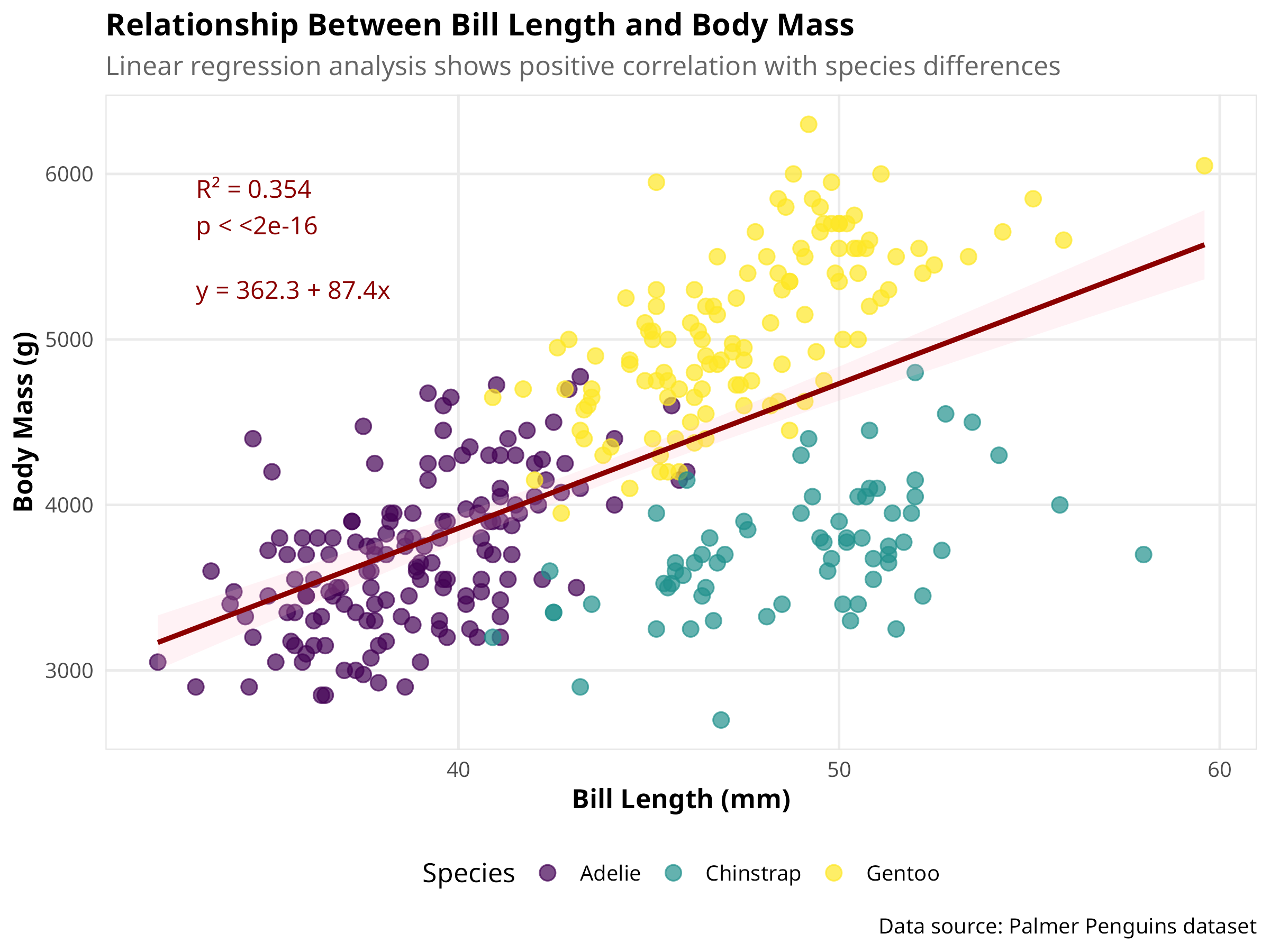
Code
# Create diagnostic plots using the performance package
check_model <- check_model(model)
plot(check_model)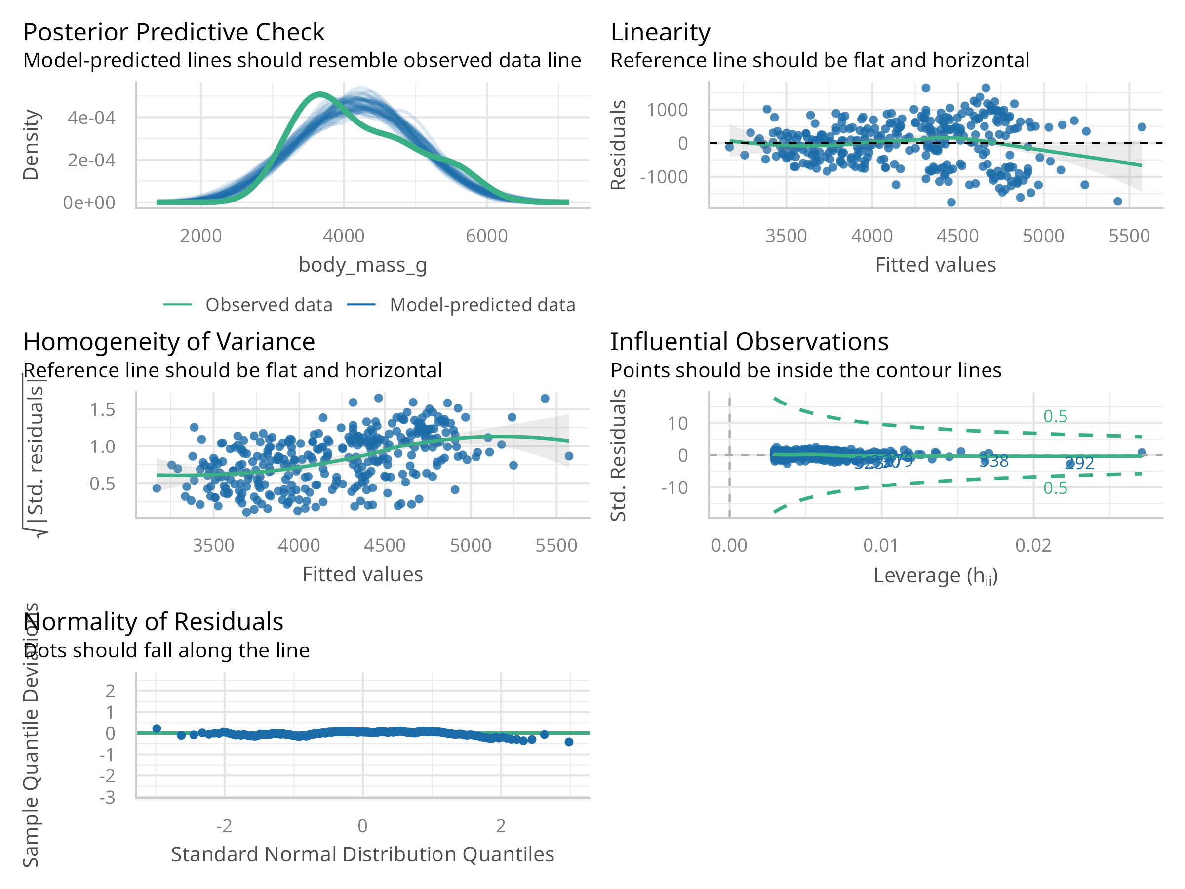
Code Explanation
This code demonstrates linear regression analysis:
-
Model Setup:
- Uses
lm()for linear regression - Predicts body mass from bill length
- Includes model diagnostics
- Uses
-
Visualization:
- Creates scatter plot with regression line
- Uses
geom_smooth()for trend line - Adds appropriate labels
-
Diagnostics:
- Residual plots
- Q-Q plot
- Scale-location plot
- Leverage plot
Results Interpretation
The regression analysis reveals:
-
Model Fit:
- Strength of relationship (R²)
- Statistical significance (p-value)
- Direction of relationship
-
Assumptions:
- Linearity of relationship
- Homogeneity of variance
- Normality of residuals
- Independence of observations
-
Practical Significance:
- Effect size
- Biological relevance
- Prediction accuracy
PROFESSIONAL TIP: Regression Analysis Best Practices
When conducting regression analysis:
-
Model Selection:
- Choose appropriate model type
- Consider variable transformations
- Check for multicollinearity
- Evaluate model assumptions
-
Diagnostic Checks:
- Examine residual plots
- Check for outliers
- Verify normality
- Assess leverage points
-
Reporting:
- Include model coefficients
- Report confidence intervals
- Provide effect sizes
- Discuss limitations
8.3 Multiple Regression
Multiple regression extends linear regression to include multiple predictors:
#> Multiple Regression Model Summary:
#> R² = 0.847, Adjusted R² = 0.845
#> F-statistic: 372.37 on 5 and 336 DF, p-value: <2e-16| term | estimate | std.error | statistic | p.value | conf.low | conf.high |
|---|---|---|---|---|---|---|
| (Intercept) | -4327.327 | 494.866 | -8.744 | 0 | -5300.752 | -3353.902 |
| bill_length_mm | 41.468 | 7.163 | 5.789 | 0 | 27.379 | 55.558 |
| bill_depth_mm | 140.328 | 18.976 | 7.395 | 0 | 103.001 | 177.655 |
| flipper_length_mm | 20.241 | 3.105 | 6.518 | 0 | 14.133 | 26.349 |
| speciesChinstrap | -513.247 | 82.140 | -6.248 | 0 | -674.819 | -351.674 |
| speciesGentoo | 934.887 | 140.778 | 6.641 | 0 | 657.971 | 1211.804 |
Code
| GVIF | Df | GVIF^(1/(2*Df)) | |
|---|---|---|---|
| bill_length_mm | 5.226 | 1 | 2.286 |
| bill_depth_mm | 4.799 | 1 | 2.191 |
| flipper_length_mm | 6.516 | 1 | 2.553 |
| species | 34.117 | 2 | 2.417 |
Code
# Check for model assumptions
check_multi_model <- check_model(multi_model)
plot(check_multi_model)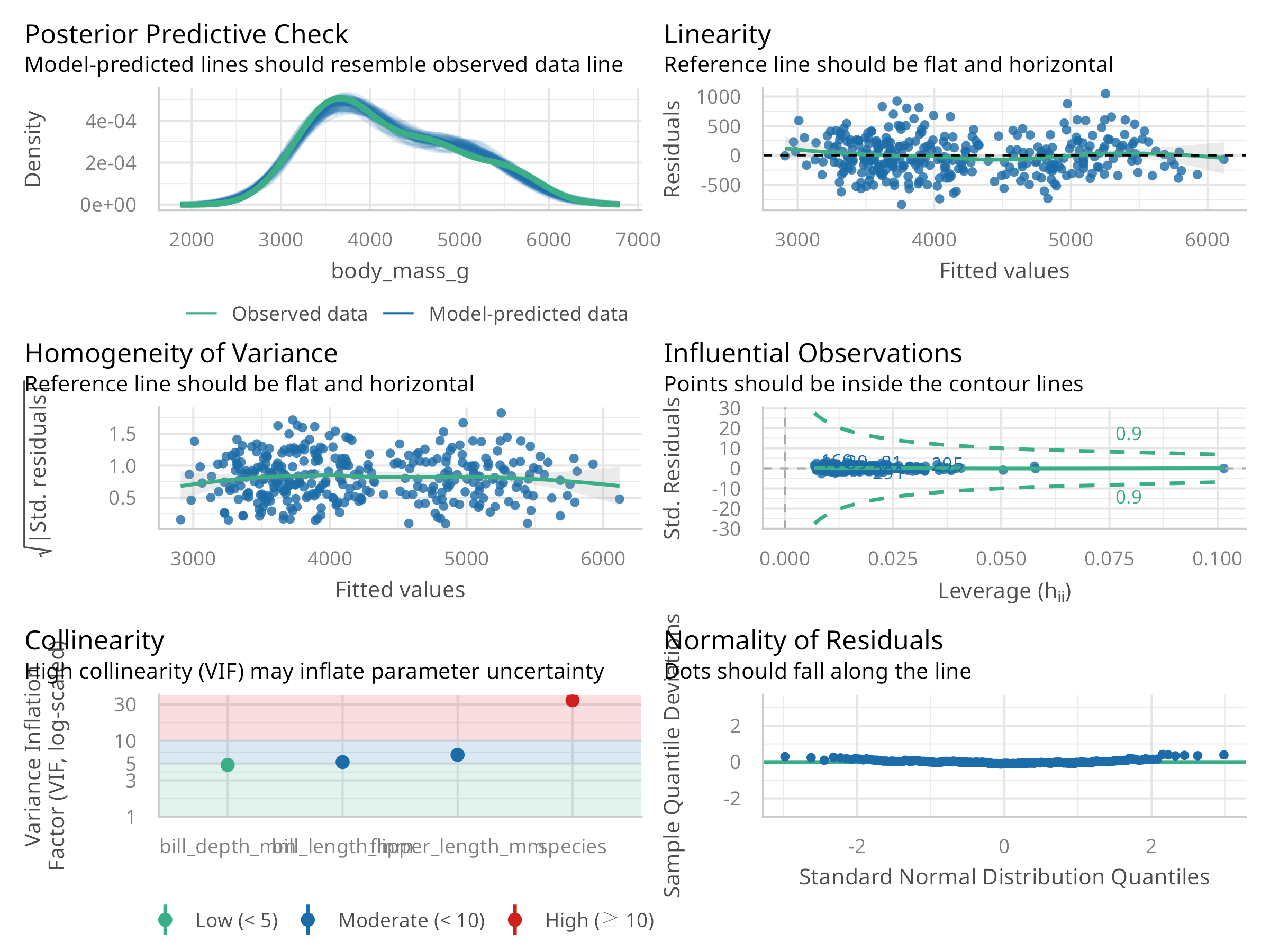
Code
# Visualize predictor effects
plot(allEffects(multi_model), ask = FALSE)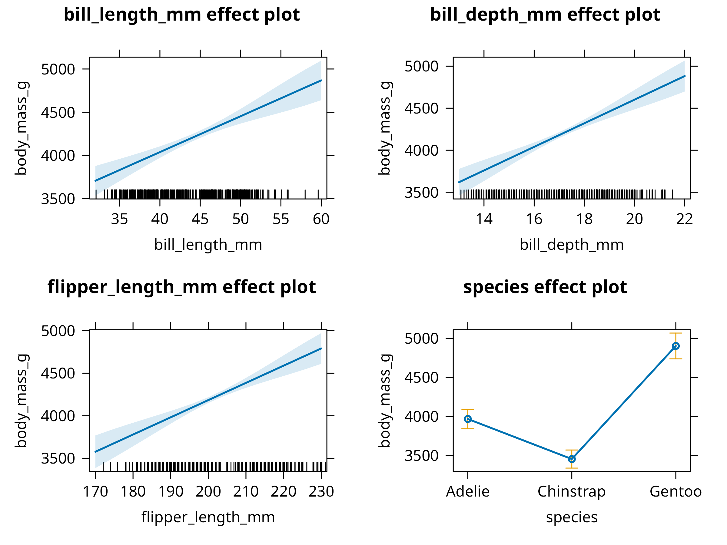
Code
# Compare models using base R
model_comparison <- data.frame(
  Metric = c("R²", "Adjusted R²", "AIC", "BIC", "N"),
  `Simple Model` = c(
    round(summary(model)$r.squared, 3),
    round(summary(model)$adj.r.squared, 3),
    round(AIC(model), 1),
    round(BIC(model), 1),
    nobs(model)
  ),
  `Multiple Model` = c(
    round(summary(multi_model)$r.squared, 3),
    round(summary(multi_model)$adj.r.squared, 3),
    round(AIC(multi_model), 1),
    round(BIC(multi_model), 1),
    nobs(multi_model)
  ),
  check.names = FALSE
)
knitr::kable(model_comparison)| Metric | Simple Model | Multiple Model |
|---|---|---|
| R² | 0.354 | 0.847 |
| Adjusted R² | 0.352 | 0.845 |
| AIC | 5400.000 | 4915.200 |
| BIC | 5411.500 | 4942.000 |
| N | 342.000 | 342.000 |
Code
# Create a visualization of predicted vs. actual values
predicted_values <- augment(multi_model, data = penguins_clean)

ggplot(predicted_values, aes(x = .fitted, y = body_mass_g, color = species)) +
  geom_point(size = 3, alpha = 0.7) +
  geom_abline(intercept = 0, slope = 1, linetype = "dashed", color = "gray50") +
  labs(
    title = "Predicted vs. Actual Body Mass",
    subtitle = "Points closer to the dashed line indicate better predictions",
    x = "Predicted Body Mass (g)",
    y = "Actual Body Mass (g)",
    color = "Species",
    caption = "Model: body_mass_g ~ bill_length_mm + bill_depth_mm + flipper_length_mm + species"
  ) +
  scale_color_viridis_d() +
  theme(legend.position = "bottom")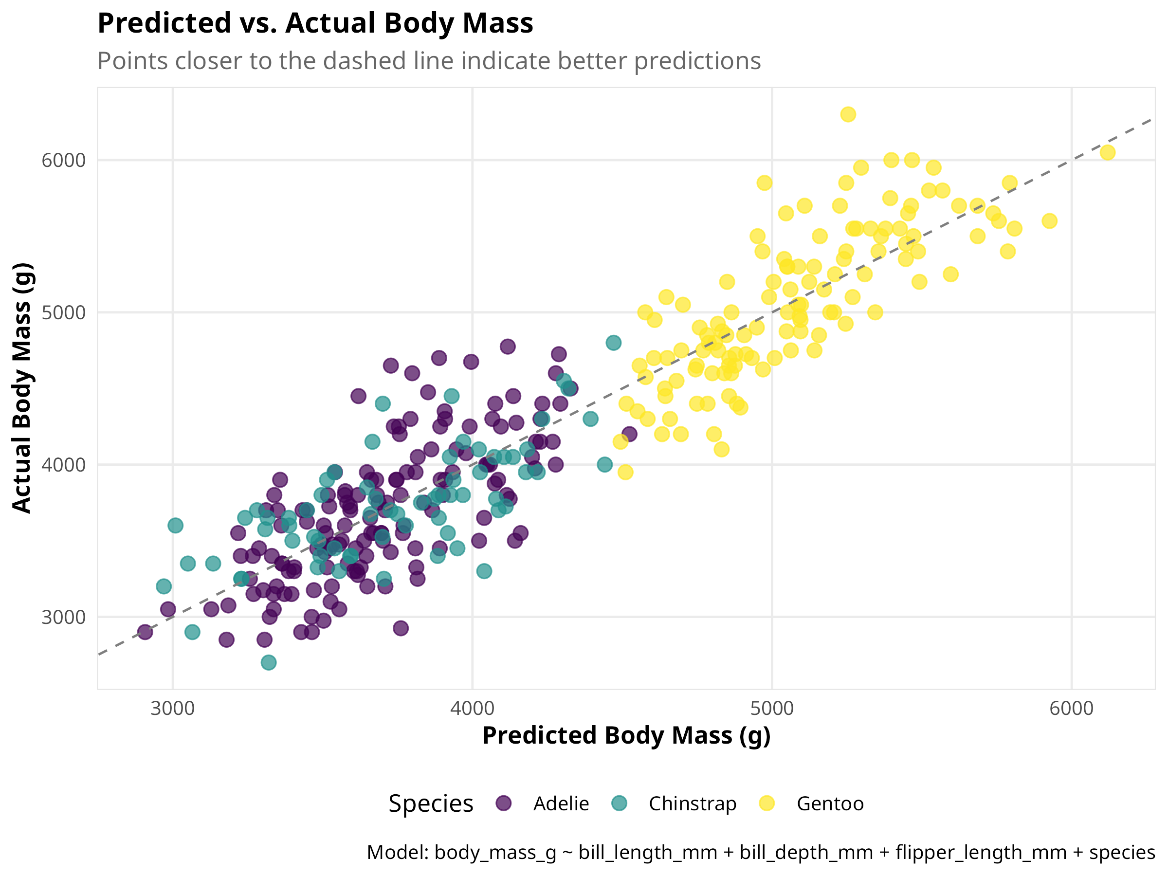
Code
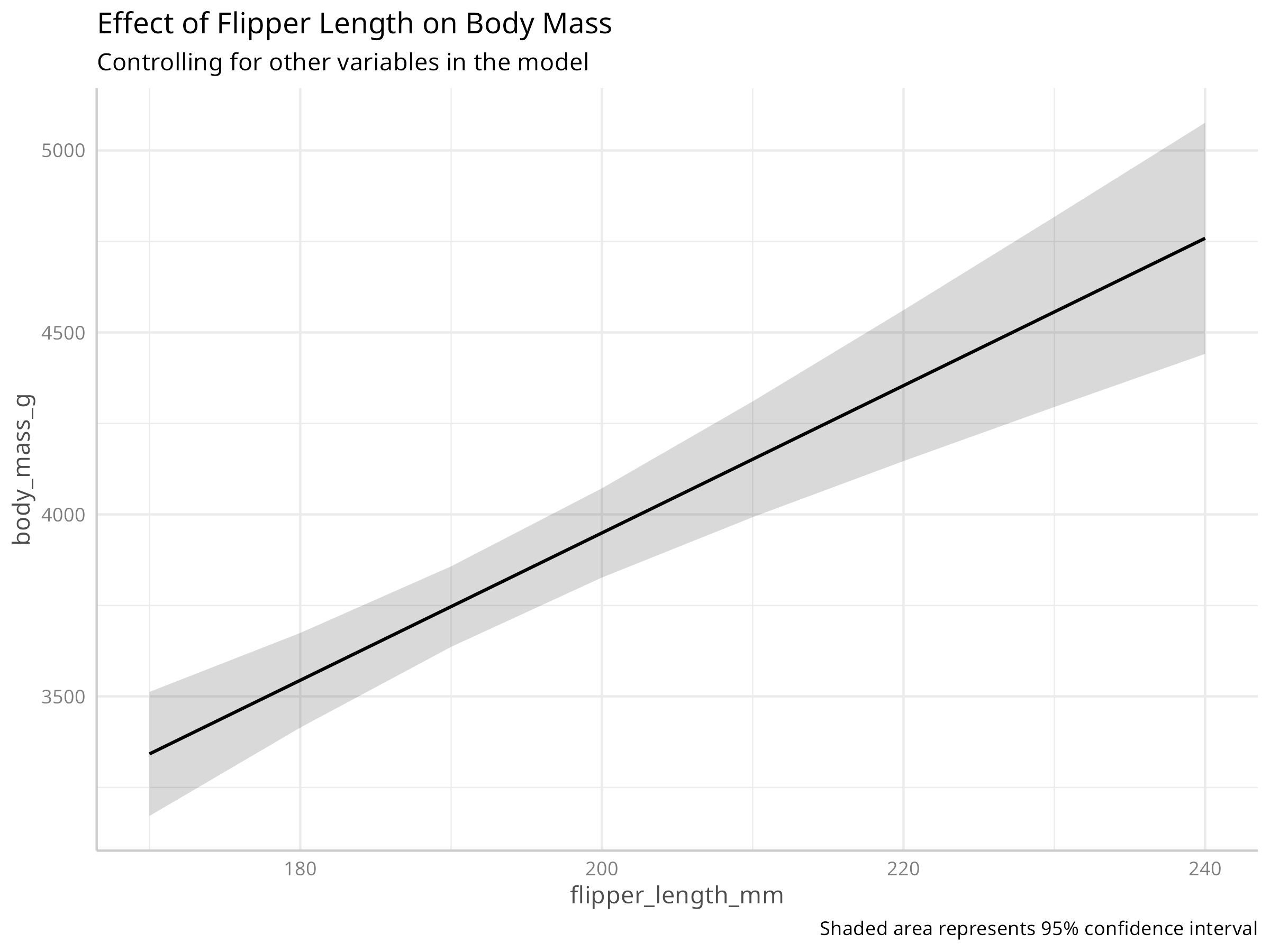
# Create a partial dependence plot for flipper length
pdp_flipper <- ggeffects::ggpredict(multi_model, terms = "flipper_length_mm")
plot(pdp_flipper) +
  labs(
    title = "Effect of Flipper Length on Body Mass",
    subtitle = "Controlling for other variables in the model",
    caption = "Shaded area represents 95% confidence interval"
  )
Code Explanation
This code demonstrates enhanced multiple regression analysis techniques:
-
Model Construction
- Uses
lm()to build a multiple regression with morphological predictors and species - Creates a more comprehensive model accounting for both measurements and taxonomy
- Properly handles categorical predictors (species) with appropriate contrasts
- Uses
-
Advanced Diagnostics
- Evaluates multicollinearity with Variance Inflation Factors (VIF)
- Conducts comprehensive model assumption checks
- Compares model performance metrics across simple and multiple regression
-
Professional Visualization
- Creates an elegant predicted vs. actual plot to assess model fit
- Generates partial dependence plots to visualize individual predictor effects
- Uses model effects plots to show relationships while controlling for other variables
- Implements consistent styling with appropriate annotations and colorblind-friendly palettes
Results Interpretation
The multiple regression analysis reveals several important insights:
-
Model Performance
- Multiple regression substantially improves explanatory power over simple regression
- The adjusted R² is much higher, indicating better model fit
- Species is a significant predictor, suggesting morphological differences between species
-
Predictor Effects
- Flipper length and bill length both positively correlate with body mass
- Species-specific effects indicate evolutionary differences in body size
- Bill depth shows a weaker relationship when controlling for other variables
-
Diagnostics Findings
- Multicollinearity (VIF values) appears manageable (VIF < 5 is generally acceptable)
- The model generally meets assumptions for inference
- Residual patterns suggest the linear model captures the main relationships well
PROFESSIONAL TIP: Multiple Regression Best Practices
When conducting ecological multiple regression analyses:
-
Model Building Strategy
- Start with biologically meaningful predictors based on theory
- Consider alternative model specifications (linear, polynomial, interactions)
- Use a hierarchical approach, starting simple and adding complexity
- Adopt information-theoretic approaches (AIC/BIC) for model selection
-
Addressing Collinearity
- Examine correlations among predictors before modeling
- Calculate VIF values and remove highly collinear predictors (VIF > 10)
- Consider dimension reduction techniques (PCA) for related predictors
- Use regularization methods (ridge, lasso) for high-dimensional data
-
Results Communication
- Present standardized coefficients to compare predictor importance
- Visualize partial effects rather than just reporting coefficients
- Report effect sizes and confidence intervals, not just p-values
- Describe both statistical and biological significance of your findings
8.4 Logistic Regression
Logistic regression models binary outcomes:
#> Logistic Regression Model Summary:
#> AIC: 23.62, Deviance: 15.62
#> Null Deviance: 469.42, DF: 341, Residual DF: 338
#> McFadden's Pseudo R²: 0.967
Code
# Create a table of odds ratios with CI
log_tidy %>%
  gt() %>%
  tab_header(title = "Logistic Regression Results (Odds Ratios)") %>%
fmt_number(columns = c("estimate", "std.error", "statistic", "p.value", "conf.low", "conf.high"), decimals = 3)| Logistic Regression Results (Odds Ratios) | ||||||
|---|---|---|---|---|---|---|
| term | estimate | std.error | statistic | p.value | conf.low | conf.high |
| (Intercept) | 44,448.176 | 15.855 | 0.675 | 0.500 | 0.000 | 92,511,770,940,489,252,864.000 |
| bill_length_mm | 0.059 | 0.970 | −2.925 | 0.003 | 0.004 | 0.224 |
| bill_depth_mm | 101.769 | 1.754 | 2.635 | 0.008 | 8.824 | 10,709.177 |
| flipper_length_mm | 1.164 | 0.094 | 1.616 | 0.106 | 0.983 | 1.467 |
Code
# Add predictions to the data
penguins_pred <- penguins_binary %>%
  mutate(
    predicted_prob = predict(log_model, type = "response"),
    predicted_class = ifelse(predicted_prob > 0.5, "Adelie", "Other"),
    correct = ifelse(predicted_class == ifelse(is_adelie == 1, "Adelie", "Other"), "Correct", "Incorrect")
  )

# Create a confusion matrix
confusion <- table(
  Predicted = penguins_pred$predicted_class,
  Actual = ifelse(penguins_pred$is_adelie == 1, "Adelie", "Other")
)

# Calculate accuracy metrics
accuracy <- sum(diag(confusion)) / sum(confusion)
sensitivity <- confusion["Adelie", "Adelie"] / sum(confusion[, "Adelie"])
specificity <- confusion["Other", "Other"] / sum(confusion[, "Other"])
precision <- confusion["Adelie", "Adelie"] / sum(confusion["Adelie", ])

# Display confusion matrix with metrics
knitr::kable(confusion,
caption = paste0("Confusion Matrix (Accuracy = ", round(accuracy * 100, 1), "%)"))| Adelie | Other | |
|---|---|---|
| Adelie | 150 | 2 |
| Other | 1 | 189 |
#> Sensitivity (True Positive Rate): 99.3%
#> Specificity (True Negative Rate): 99%
#> Precision (Positive Predictive Value): 98.7%
Code
Code
# Create a visualization of predicted probabilities by species
ggplot(penguins_pred, aes(x = bill_depth_mm, y = body_mass_g, color = predicted_prob)) +
  geom_point(size = 3, alpha = 0.7) +
  # Add decision boundary (0.5 probability contour)
  geom_contour(aes(z = predicted_prob), breaks = 0.5, color = "black", linewidth = 1) +
  # Add text labels for misclassified points
  geom_text(data = filter(penguins_pred, correct == "Incorrect"),
            aes(label = "✗"), color = "black", size = 4, nudge_y = 0.5) +
  # Color gradient for probability
  scale_color_gradient2(low = "navy", mid = "white", high = "red",
                      midpoint = 0.5, limits = c(0, 1)) +
  facet_wrap(~species) +
  labs(
    title = "Classification of Adelie vs. Other Penguins",
    subtitle = paste0("AUC = ", round(auc_value, 3), ", Accuracy = ", round(accuracy * 100, 1), "%"),
    x = "Bill Depth (mm)",
    y = "Body Mass (g)",
    color = "Probability\nof Adelie",
    caption = "Black line: decision boundary (p=0.5), ✗: misclassified points"
  ) +
  theme(legend.position = "right")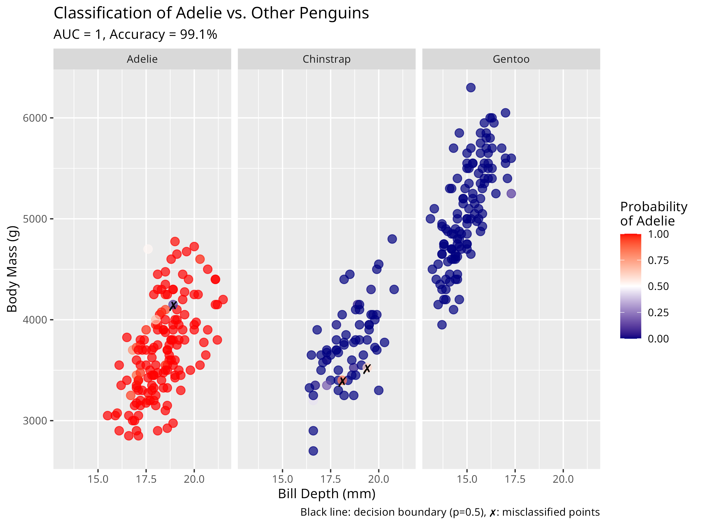
Code
# Create marginal effects plots for the predictors
plot(allEffects(log_model), ask = FALSE, main = "Marginal Effects on Probability of Adelie")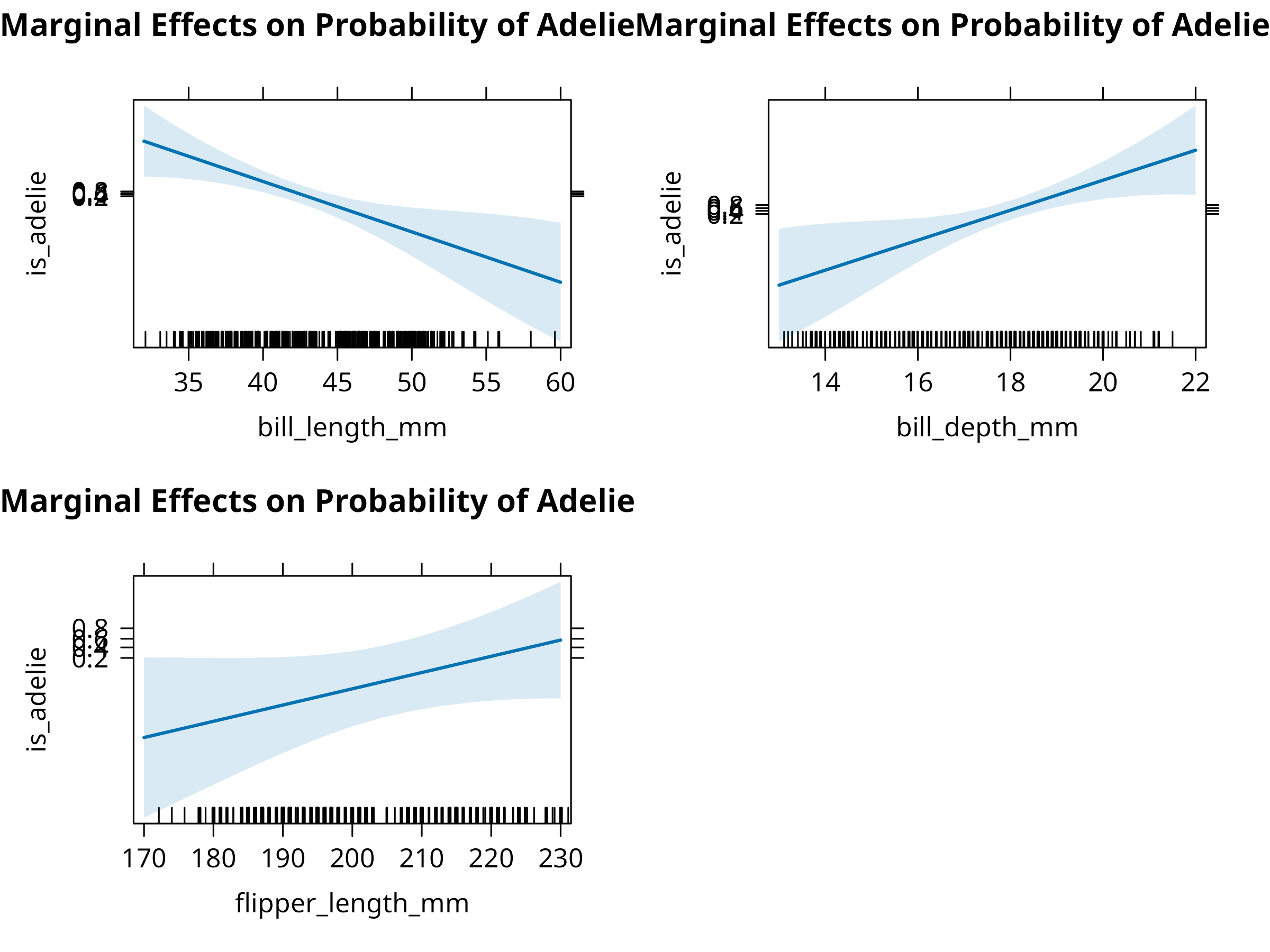
Code
# Check model fit
sim_residuals <- simulateResiduals(log_model)
plot(sim_residuals)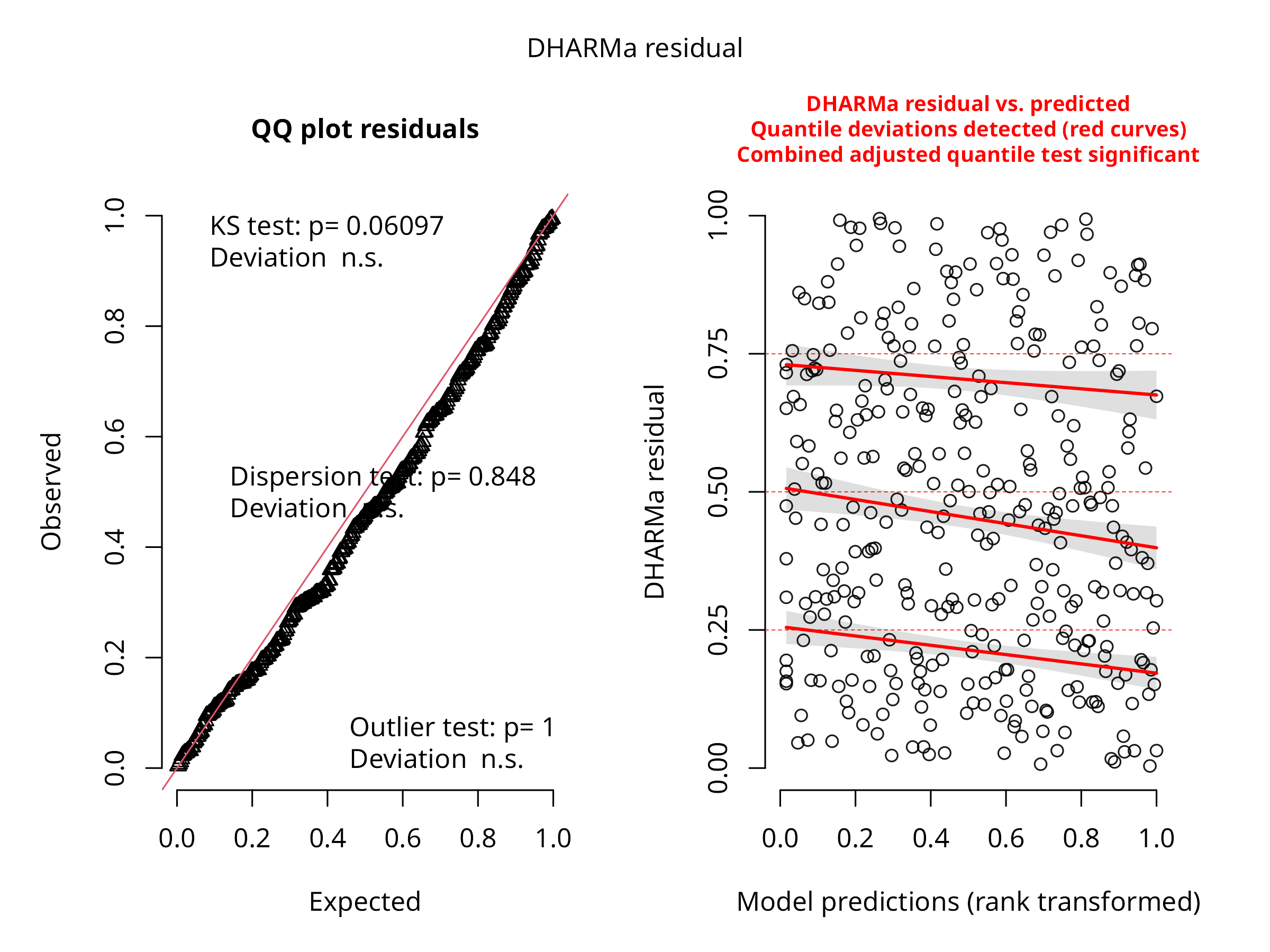
Code Explanation
This enhanced logistic regression analysis provides comprehensive insights:
-
Model Construction
- Creates a binary outcome variable (Adelie vs. Other species)
- Uses
glm()with a binomial family and logit link - Incorporates multiple predictors (bill depth, body mass)
-
Professional Reporting
- Displays odds ratios with confidence intervals for interpretability
- Calculates and reports pseudo-R² (McFadden) for model fit
- Creates a detailed confusion matrix with classification metrics
- Generates a ROC curve with AUC for overall discriminative ability
-
Advanced Visualization
- Plots predicted probabilities with decision boundaries
- Highlights misclassified points for error analysis
- Creates marginal effects plots showing how each predictor influences classification
- Conducts simulation-based residual analysis for model validation
Results Interpretation
The logistic regression yields important ecological insights:
-
Classification Performance
- The model effectively distinguishes Adelie penguins from other species
- High AUC (area under ROC curve) indicates strong discriminative ability
- Classification accuracy, sensitivity, and specificity show the practical utility
-
Morphological Predictors
- Bill dimensions are strong predictors of species identity
- Odds ratios reveal how changes in morphology affect classification probability
- Interaction between bill length and depth creates a clear decision boundary
-
Ecological Implications
- The model demonstrates morphological differentiation between penguin species
- Misclassified individuals may represent morphological overlap zones
- Results align with evolutionary theory on character displacement
- Potential applications in field identification and evolutionary studies
PROFESSIONAL TIP: Logistic Regression Best Practices
When applying logistic regression in ecological studies:
-
Model Development
- Balance the number of events and predictors (aim for >10 events per predictor)
- Test for nonlinearity in continuous predictors using splines or polynomial terms
- Evaluate interactions between predictors where biologically meaningful
- Consider regularization for high-dimensional data to prevent overfitting
-
Model Evaluation
- Use cross-validation to assess predictive performance
- Report multiple performance metrics beyond p-values (AUC, accuracy, sensitivity, specificity)
- Consider the costs of different error types (false positives vs. false negatives)
- Test model calibration (agreement between predicted probabilities and observed outcomes)
-
Result Communication
- Report odds ratios for interpretability (not just coefficients)
- Create visualizations showing decision boundaries and classification regions
- Discuss practical significance for ecological applications
- Indicate model limitations and potential sampling biases
8.5 Summary
In this chapter, we’ve explored regression analysis using both traditional base R approaches and the modern tidymodels framework:
- Linear regression for modeling continuous relationships between morphological variables
- Multiple regression for incorporating several predictors and controlling for confounding factors
- Logistic regression for binary classification and probability estimation
- Tidymodels workflow for consistent, reproducible modeling
The tidymodels framework provides: - Unified interface across different model types - Consistent preprocessing with recipes - Built-in resampling and cross-validation - Standardized model evaluation metrics - Streamlined workflow management
Each approach provides unique insights into ecological patterns and relationships, with applications ranging from morphological studies to species classification and trait prediction.
8.6 Regression with Tidymodels Framework
The tidymodels ecosystem provides a modern, unified approach to statistical modeling in R. Let’s explore how to implement regression analysis using this framework.
8.6.1 Setting Up Tidymodels
Code
# Load tidymodels packages
library(tidymodels)  # Meta-package loading parsnip, recipes, rsample, tune, workflows, yardstick
library(tidyverse)    # For data manipulation

# Set random seed for reproducibility
set.seed(123)

# Load and prepare data
penguins <- read_csv("../data/environmental/climate_data.csv", show_col_types = FALSE) %>%
  filter(!is.na(bill_length_mm), !is.na(body_mass_g),
         !is.na(bill_depth_mm), !is.na(flipper_length_mm)) %>%
  mutate(species = as.factor(species))

# Display data structure
glimpse(penguins)
#> Rows: 342
#> Columns: 8
#> $ species           <fct> Adelie, Adelie, Adelie, Adelie, Adelie, Adelie, Adel…
#> $ island            <chr> "Torgersen", "Torgersen", "Torgersen", "Torgersen", …
#> $ bill_length_mm    <dbl> 39.1, 39.5, 40.3, 36.7, 39.3, 38.9, 39.2, 34.1, 42.0…
#> $ bill_depth_mm     <dbl> 18.7, 17.4, 18.0, 19.3, 20.6, 17.8, 19.6, 18.1, 20.2…
#> $ flipper_length_mm <dbl> 181, 186, 195, 193, 190, 181, 195, 193, 190, 186, 18…
#> $ body_mass_g       <dbl> 3750, 3800, 3250, 3450, 3650, 3625, 4675, 3475, 4250…
#> $ sex               <chr> "male", "female", "female", "female", "male", "femal…
#> $ year              <dbl> 2007, 2007, 2007, 2007, 2007, 2007, 2007, 2007, 2007…
Tidymodels Philosophy
The tidymodels framework follows key principles:
- Consistency: Uniform syntax across different model types
- Modularity: Separate components for different modeling tasks
- Tidyverse integration: Works seamlessly with dplyr, ggplot2, etc.
- Reproducibility: Built-in support for resampling and validation
- Extensibility: Easy to add new models and methods
8.6.2 Linear Regression with Tidymodels
Code
# Step 1: Split data into training and testing sets
penguin_split <- initial_split(penguins, prop = 0.75, strata = species)
penguin_train <- training(penguin_split)
penguin_test <- testing(penguin_split)

cat("Training set:", nrow(penguin_train), "observations\n")
#> Training set: 256 observations
cat("Testing set:", nrow(penguin_test), "observations\n")
#> Testing set: 86 observations

# Step 2: Define a recipe for preprocessing
penguin_recipe <- recipe(body_mass_g ~ bill_length_mm + bill_depth_mm +
                         flipper_length_mm + species,
                         data = penguin_train) %>%
  step_dummy(species) %>%
  step_normalize(all_numeric_predictors()) %>%
  step_zv(all_predictors())

# Step 3: Specify the model
lm_spec <- linear_reg() %>%
  set_engine("lm") %>%
  set_mode("regression")

# Step 4: Create a workflow combining recipe and model
penguin_wf <- workflow() %>%
  add_recipe(penguin_recipe) %>%
  add_model(lm_spec)

# Step 5: Fit the model
penguin_fit <- penguin_wf %>%
fit(data = penguin_train)| term | estimate | std.error | statistic | p.value |
|---|---|---|---|---|
| (Intercept) | 4191.992 | 20.678 | 202.725 | 0 |
| bill_length_mm | 267.541 | 50.646 | 5.283 | 0 |
| bill_depth_mm | 278.664 | 46.447 | 6.000 | 0 |
| flipper_length_mm | 243.626 | 53.809 | 4.528 | 0 |
| species_Chinstrap | -236.669 | 42.184 | -5.610 | 0 |
| species_Gentoo | 450.673 | 82.451 | 5.466 | 0 |
Code
| .metric | .estimator | .estimate |
|---|---|---|
| rmse | standard | 326.952 |
| rsq | standard | 0.832 |
| mae | standard | 260.412 |
Code
| .metric | .estimator | .estimate |
|---|---|---|
| rmse | standard | 272.490 |
| rsq | standard | 0.888 |
| mae | standard | 216.419 |
Code
penguin_pred <- penguin_fit %>%
  predict(penguin_test) %>%
  bind_cols(penguin_test)

ggplot(penguin_pred, aes(x = body_mass_g, y = .pred, color = species)) +
  geom_point(size = 3, alpha = 0.7) +
  geom_abline(slope = 1, intercept = 0, linetype = "dashed", color = "gray50") +
  scale_color_viridis_d() +
  labs(
    title = "Tidymodels: Predicted vs. Actual Body Mass",
    subtitle = "Test set predictions from linear regression workflow",
    x = "Actual Body Mass (g)",
    y = "Predicted Body Mass (g)",
    color = "Species",
    caption = "Dashed line represents perfect predictions"
  ) +
  theme_minimal()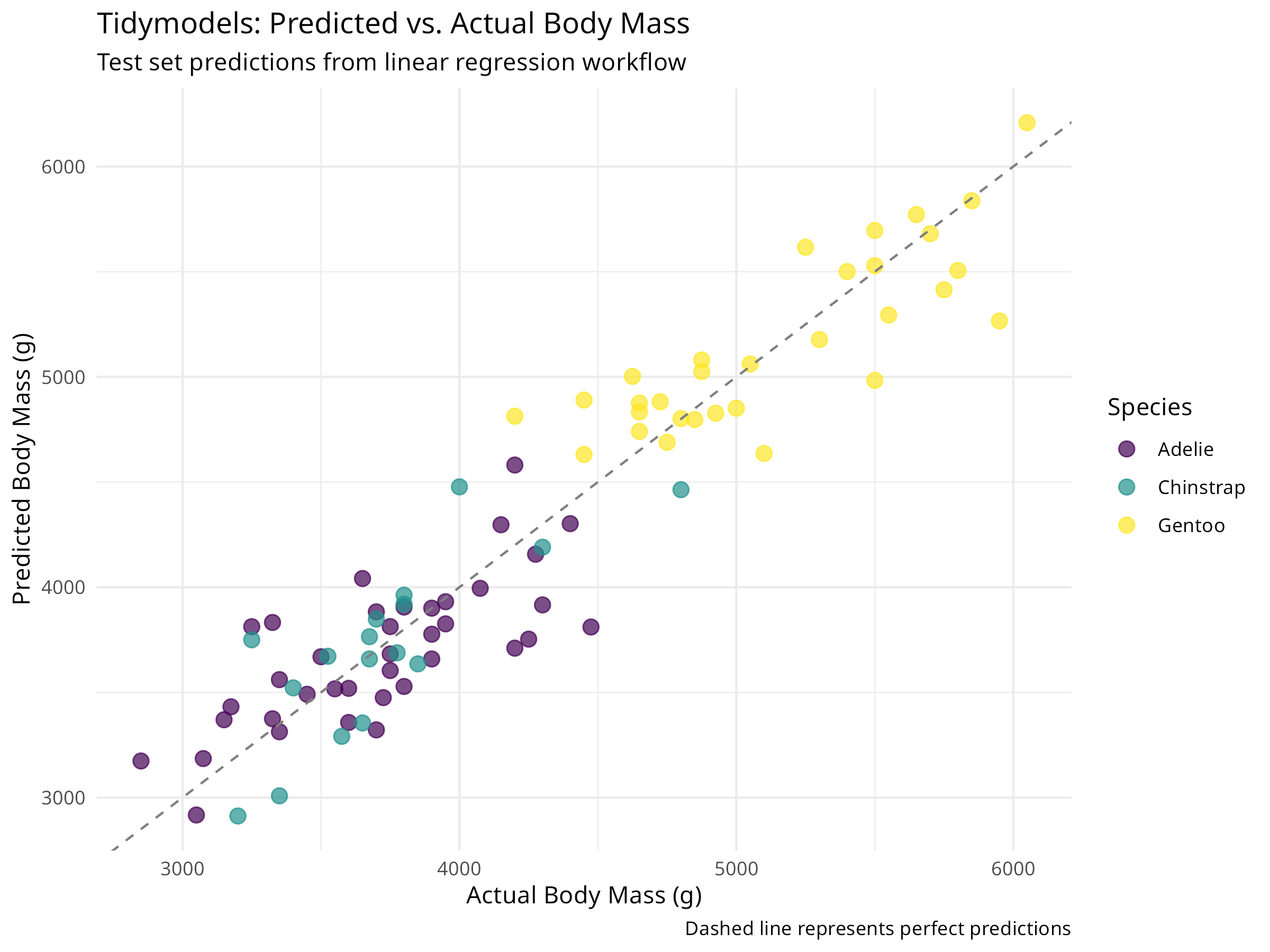
Tidymodels Workflow Benefits
This tidymodels approach provides several advantages:
- Clear separation of concerns: Data splitting, preprocessing, and modeling are distinct steps
- Automatic train/test split: Built-in support for validation
- Preprocessing pipeline: Recipe ensures consistent transformations
- Reusable workflows: Easy to apply the same pipeline to new data
- Standardized metrics: Consistent evaluation across models
The test set RMSE and R² provide unbiased estimates of model performance on new data.
8.6.3 Cross-Validation with Tidymodels
Code
# Create cross-validation folds
set.seed(456)
penguin_folds <- vfold_cv(penguin_train, v = 10, strata = species)

cat("Created", nrow(penguin_folds), "cross-validation folds\n")
#> Created 10 cross-validation folds

# Fit model using cross-validation
cv_results <- penguin_wf %>%
  fit_resamples(
    resamples = penguin_folds,
    control = control_resamples(save_pred = TRUE),
    metrics = metric_set(rmse, rsq, mae)
  )
Code
cv_metrics <- collect_metrics(cv_results)
knitr::kable(cv_metrics, digits = 3)| .metric | .estimator | mean | n | std_err | .config |
|---|---|---|---|---|---|
| mae | standard | 267.534 | 10 | 11.696 | pre0_mod0_post0 |
| rmse | standard | 334.650 | 10 | 11.419 | pre0_mod0_post0 |
| rsq | standard | 0.832 | 10 | 0.016 | pre0_mod0_post0 |
Code
collect_metrics(cv_results, summarize = FALSE) %>%
  ggplot(aes(x = .metric, y = .estimate)) +
  geom_boxplot(fill = "skyblue", alpha = 0.7) +
  geom_jitter(width = 0.1, alpha = 0.5, size = 2) +
  labs(
    title = "Cross-Validation Performance Distribution",
    subtitle = "10-fold CV shows model stability across folds",
    x = "Metric",
    y = "Value"
  ) +
  theme_minimal()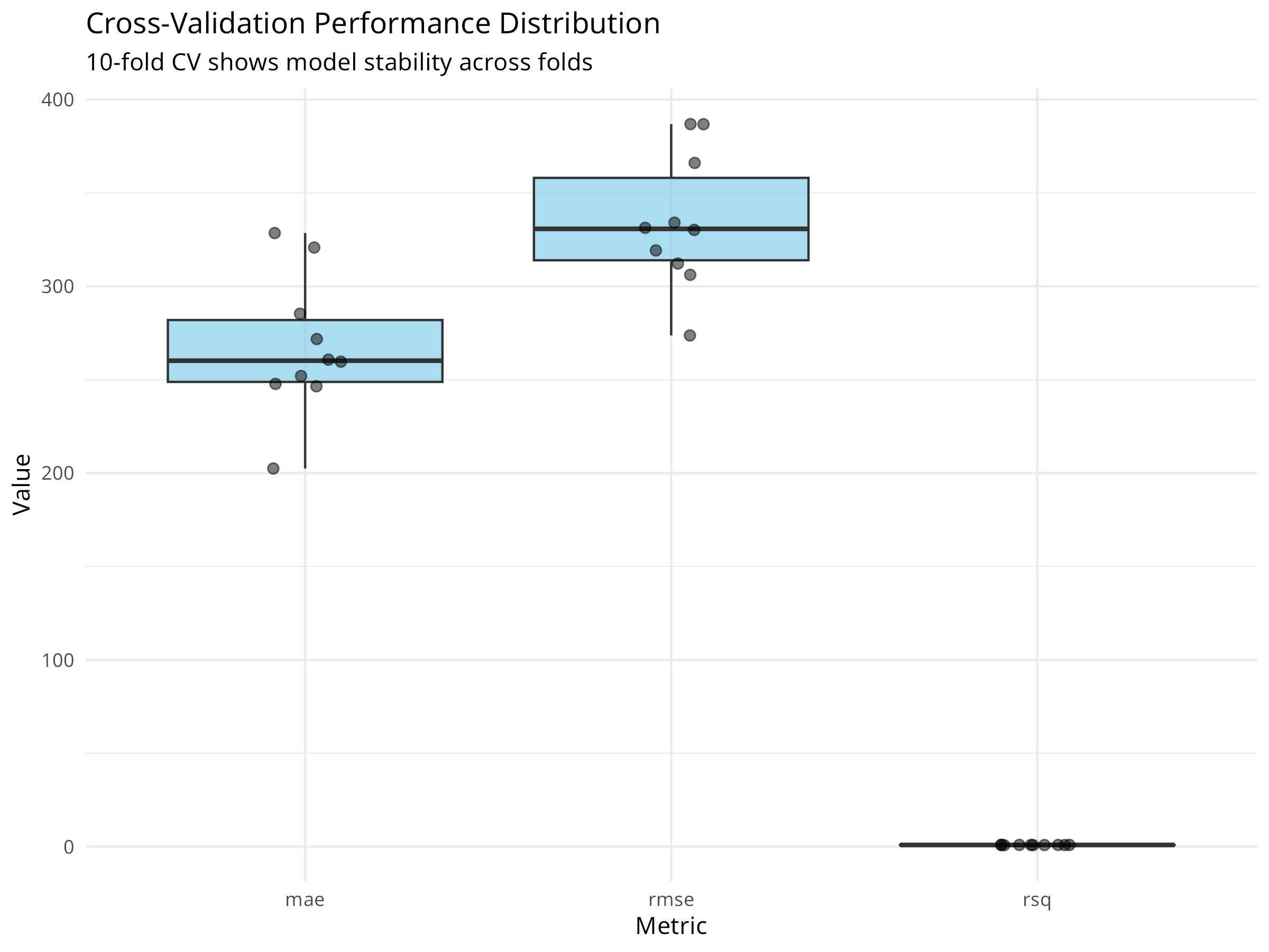
Code
cv_predictions <- collect_predictions(cv_results)

ggplot(cv_predictions, aes(x = body_mass_g, y = .pred)) +
  geom_point(alpha = 0.5, color = "steelblue") +
  geom_abline(slope = 1, intercept = 0, linetype = "dashed", color = "red") +
  labs(
    title = "Cross-Validation Predictions",
    subtitle = "All predictions from 10-fold CV",
    x = "Actual Body Mass (g)",
    y = "Predicted Body Mass (g)"
  ) +
  theme_minimal()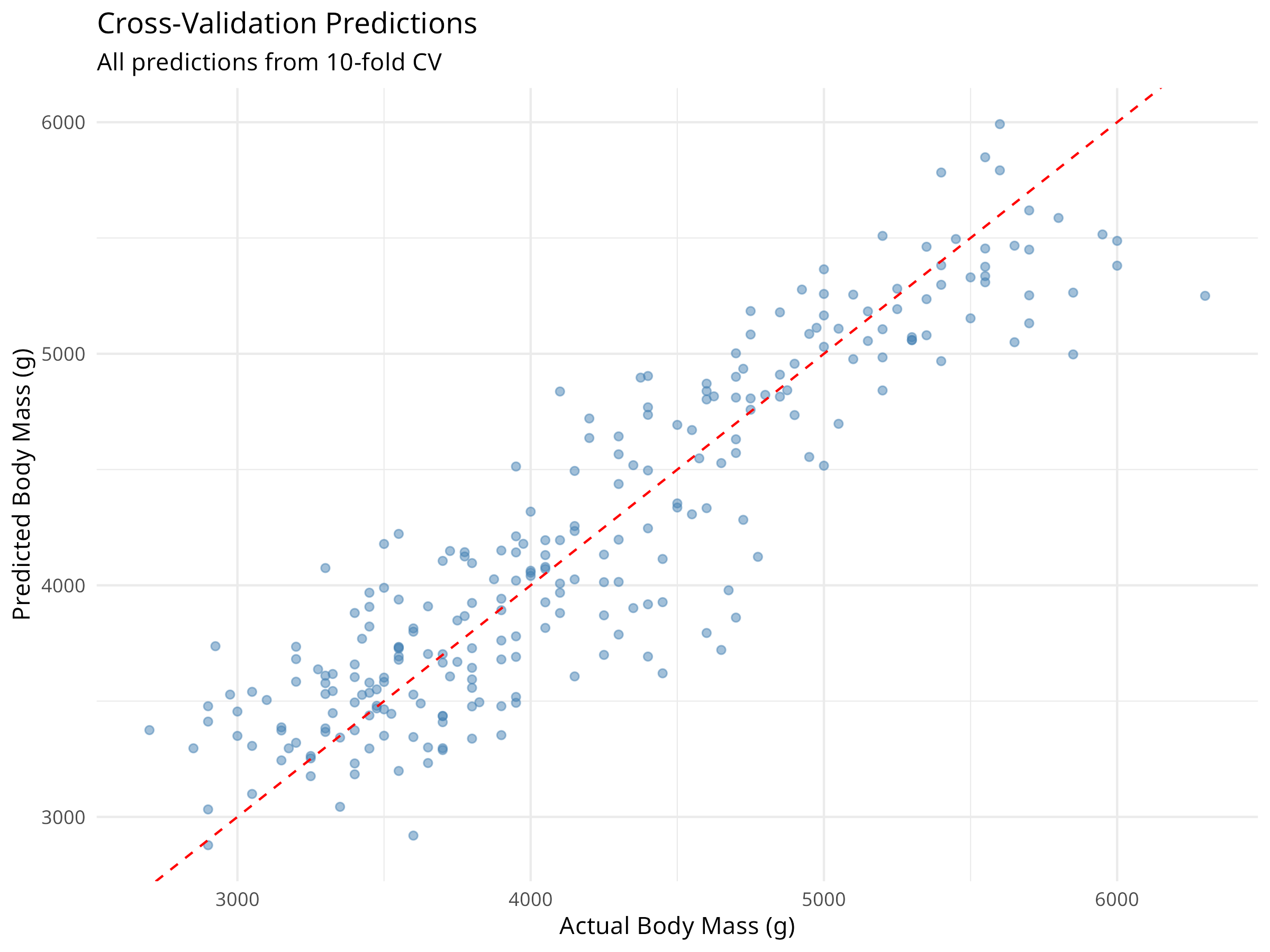
PROFESSIONAL TIP: Why Cross-Validation?
Cross-validation provides:
- More reliable performance estimates: Averages over multiple train/test splits
- Better use of data: All observations used for both training and validation
- Overfitting detection: Large difference between training and CV metrics suggests overfitting
- Model comparison: Fair basis for comparing different modeling approaches
- Hyperparameter tuning: Essential for selecting optimal model parameters
8.6.4 Model Comparison with Tidymodels
Code
# Define multiple model specifications
lm_spec <- linear_reg() %>%
  set_engine("lm") %>%
  set_mode("regression")

rf_spec <- rand_forest(trees = 100) %>%
  set_engine("ranger") %>%
  set_mode("regression")

# Create workflows for each model
lm_wf <- workflow() %>%
  add_recipe(penguin_recipe) %>%
  add_model(lm_spec)

rf_wf <- workflow() %>%
  add_recipe(penguin_recipe) %>%
  add_model(rf_spec)

# Fit both models with cross-validation
set.seed(789)
lm_cv <- lm_wf %>%
  fit_resamples(
    resamples = penguin_folds,
    metrics = metric_set(rmse, rsq, mae)
  )

rf_cv <- rf_wf %>%
  fit_resamples(
    resamples = penguin_folds,
    metrics = metric_set(rmse, rsq, mae)
  )

# Compare model performance
model_comparison <- bind_rows(
  collect_metrics(lm_cv) %>% mutate(model = "Linear Regression"),
  collect_metrics(rf_cv) %>% mutate(model = "Random Forest")
)
Code
| Model | Metric | Mean | Std Error |
|---|---|---|---|
| Linear Regression | mae | 267.534 | 11.696 |
| Linear Regression | rmse | 334.650 | 11.419 |
| Linear Regression | rsq | 0.832 | 0.016 |
| Random Forest | mae | 275.905 | 13.512 |
| Random Forest | rmse | 351.537 | 11.963 |
| Random Forest | rsq | 0.811 | 0.020 |
Code
model_comparison %>%
  ggplot(aes(x = model, y = mean, fill = model)) +
  geom_col() +
  geom_errorbar(aes(ymin = mean - std_err, ymax = mean + std_err),
                width = 0.2) +
  facet_wrap(~ .metric, scales = "free_y") +
  scale_fill_viridis_d(begin = 0.3, end = 0.8) +
  labs(
    title = "Model Performance Comparison",
    subtitle = "Cross-validation results with standard errors",
    x = "Model Type",
    y = "Performance (mean ± SE)"
  ) +
  theme_minimal() +
  theme(legend.position = "none",
        axis.text.x = element_text(angle = 45, hjust = 1))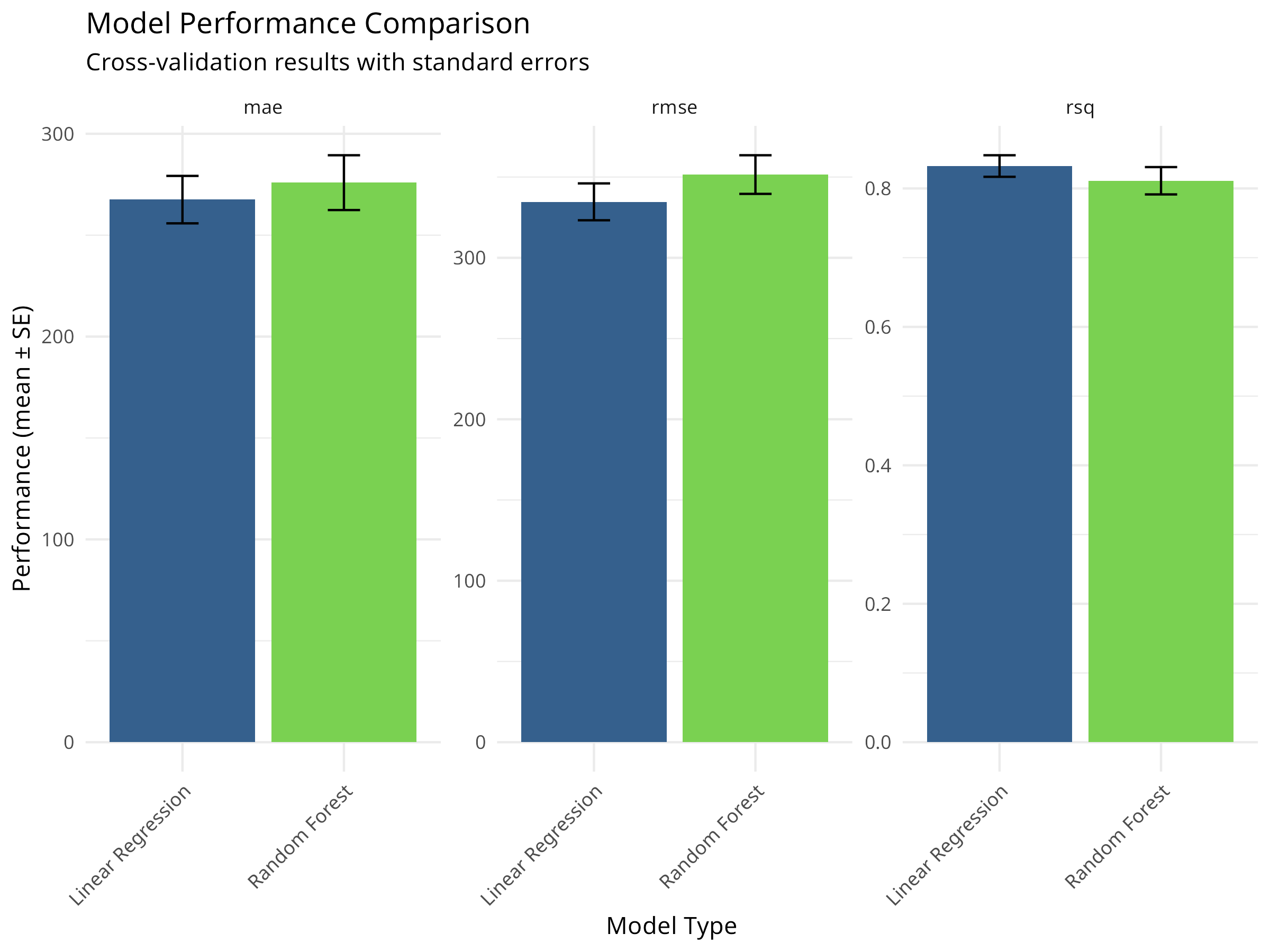
8.6.5 Hyperparameter Tuning
Optimizing model parameters is crucial for machine learning models like Random Forest.
Code
# Define a model specification with tunable parameters
rf_tune_spec <- rand_forest(
  trees = 1000,
  mtry = tune(),
  min_n = tune()
) %>%
  set_engine("ranger") %>%
  set_mode("regression")

# Create a workflow with the tunable model
rf_tune_wf <- workflow() %>%
  add_recipe(penguin_recipe) %>%
  add_model(rf_tune_spec)

# Define the grid of parameter values to try
rf_grid <- grid_regular(
  mtry(range = c(1, 5)),
  min_n(range = c(2, 10)),
  levels = 5
)

# Tune the model using cross-validation
# Note: This may take a moment to run
set.seed(345)
rf_tune_res <- tune_grid(
  rf_tune_wf,
  resamples = penguin_folds,
  grid = rf_grid,
  metrics = metric_set(rmse, rsq)
)

# Collect tuning metrics
rf_tune_res %>%
  collect_metrics() %>%
  filter(.metric == "rmse") %>%
  pivot_longer(cols = c(mtry, min_n), names_to = "parameter", values_to = "value") %>%
  ggplot(aes(x = value, y = mean, color = parameter)) +
  geom_point() +
  geom_line() +
  facet_wrap(~parameter, scales = "free_x") +
  labs(title = "Hyperparameter Tuning Results", y = "RMSE (lower is better)") +
  theme_minimal()

# Select the best parameters
best_rf <- select_best(rf_tune_res, metric = "rmse")
print(best_rf)
#> # A tibble: 1 × 3
#>    mtry min_n .config
#>   <int> <int> <chr>
#> 1     2    10 pre0_mod10_post0

# Finalize the workflow with the best parameters
final_rf_wf <- finalize_workflow(rf_tune_wf, best_rf)

# Fit the final model to the full training set and evaluate on test set
final_fit <- last_fit(final_rf_wf, penguin_split)

# Show final performance
collect_metrics(final_fit)
#> # A tibble: 2 × 4
#>   .metric .estimator .estimate .config
#>   <chr>   <chr>          <dbl> <chr>
#> 1 rmse    standard     291.    pre0_mod0_post0
#> 2 rsq     standard       0.872 pre0_mod0_post0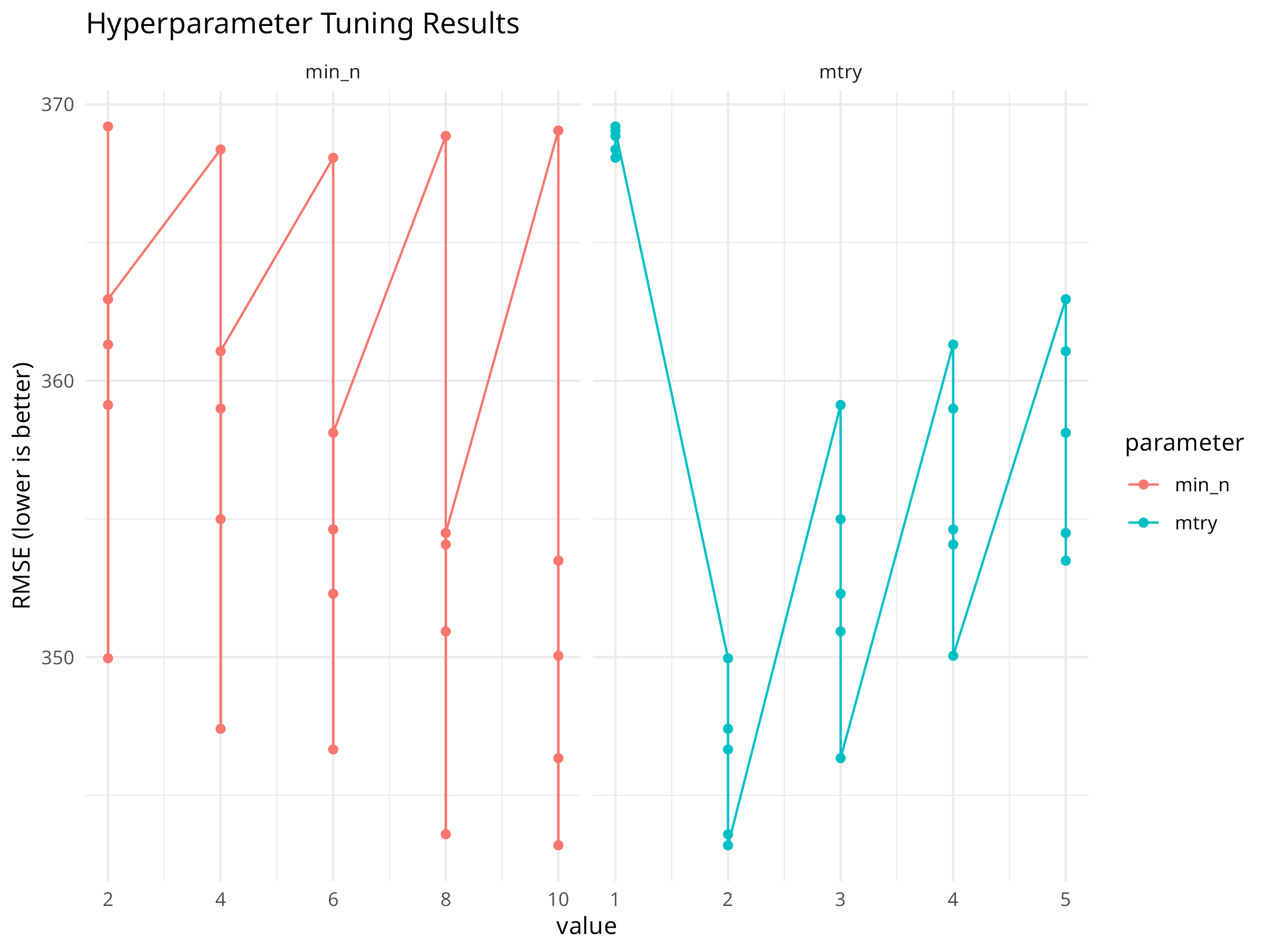
Tuning Strategy
Grid search explores a defined set of parameters. For more complex models, consider tune_bayes() for Bayesian optimization which can be more efficient.
8.7 Chapter Summary
8.7.1 Key Concepts
- Linear Regression: Models continuous outcomes as a linear combination of predictors
- Logistic Regression: Models binary outcomes using the log-odds transformation
- Tidymodels: A unified framework for modeling in R (parsnip, recipes, rsample, tune, yardstick)
- Cross-Validation: Resampling method to estimate model performance on unseen data
- Hyperparameter Tuning: Optimizing model configuration to improve predictive power
- Model Diagnostics: Checking assumptions (normality, homoscedasticity, linearity) is essential
8.7.2 R Functions Learned
-
lm()/glm()- Base R regression functions -
linear_reg()/logistic_reg()/rand_forest()- Parsnip model specifications -
recipe()- Define preprocessing steps -
vfold_cv()- Create cross-validation folds -
fit_resamples()- Evaluate models with resampling -
tune_grid()- Optimize hyperparameters -
collect_metrics()- Extract performance statistics
8.7.3 Next Steps
In the next chapter, we will explore Advanced Modeling Techniques, including how to interpret complex “black box” models and how to analyze data collected over time (time series).
8.7.4 Logistic Regression with Tidymodels
Code
# Prepare binary classification data
penguins_binary <- penguins %>%
  mutate(is_adelie = factor(ifelse(species == "Adelie", "Adelie", "Other"),
                           levels = c("Other", "Adelie")))

# Split data
set.seed(2023)
binary_split <- initial_split(penguins_binary, prop = 0.75, strata = is_adelie)
binary_train <- training(binary_split)
binary_test <- testing(binary_split)

# Create recipe
logistic_recipe <- recipe(is_adelie ~ bill_depth_mm + body_mass_g,
                         data = binary_train) %>%
  step_normalize(all_numeric_predictors())

# Specify logistic regression model
logistic_spec <- logistic_reg() %>%
  set_engine("glm") %>%
  set_mode("classification")

# Create workflow
logistic_wf <- workflow() %>%
  add_recipe(logistic_recipe) %>%
  add_model(logistic_spec)

# Fit the model
logistic_fit <- logistic_wf %>%
  fit(data = binary_train)

# Get predictions with probabilities
logistic_pred <- logistic_fit %>%
  predict(binary_test, type = "prob") %>%
  bind_cols(logistic_fit %>% predict(binary_test)) %>%
  bind_cols(binary_test)
Code
| .metric | .estimator | .estimate |
|---|---|---|
| accuracy | binary | 0.988 |
| kap | binary | 0.976 |
| mn_log_loss | binary | 15.979 |
| roc_auc | binary | 0.000 |
Code
conf_mat(logistic_pred, truth = is_adelie, estimate = .pred_class) %>%
  autoplot(type = "heatmap") +
  labs(title = "Confusion Matrix: Adelie Classification") +
  theme_minimal()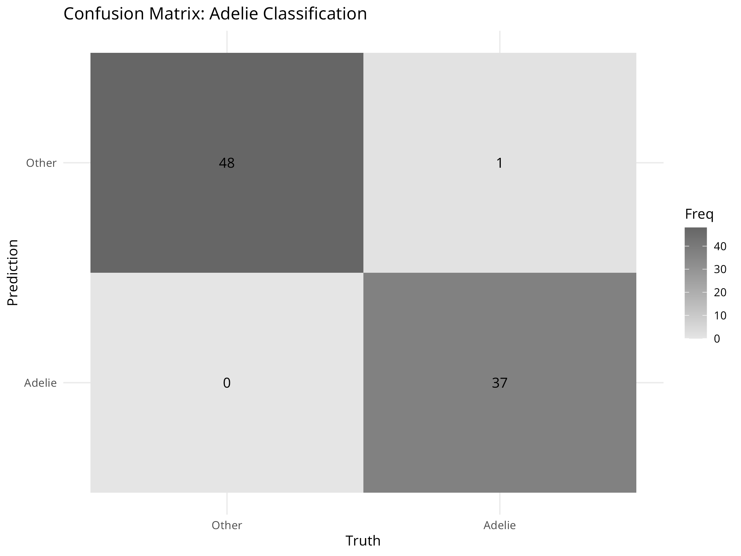
Code
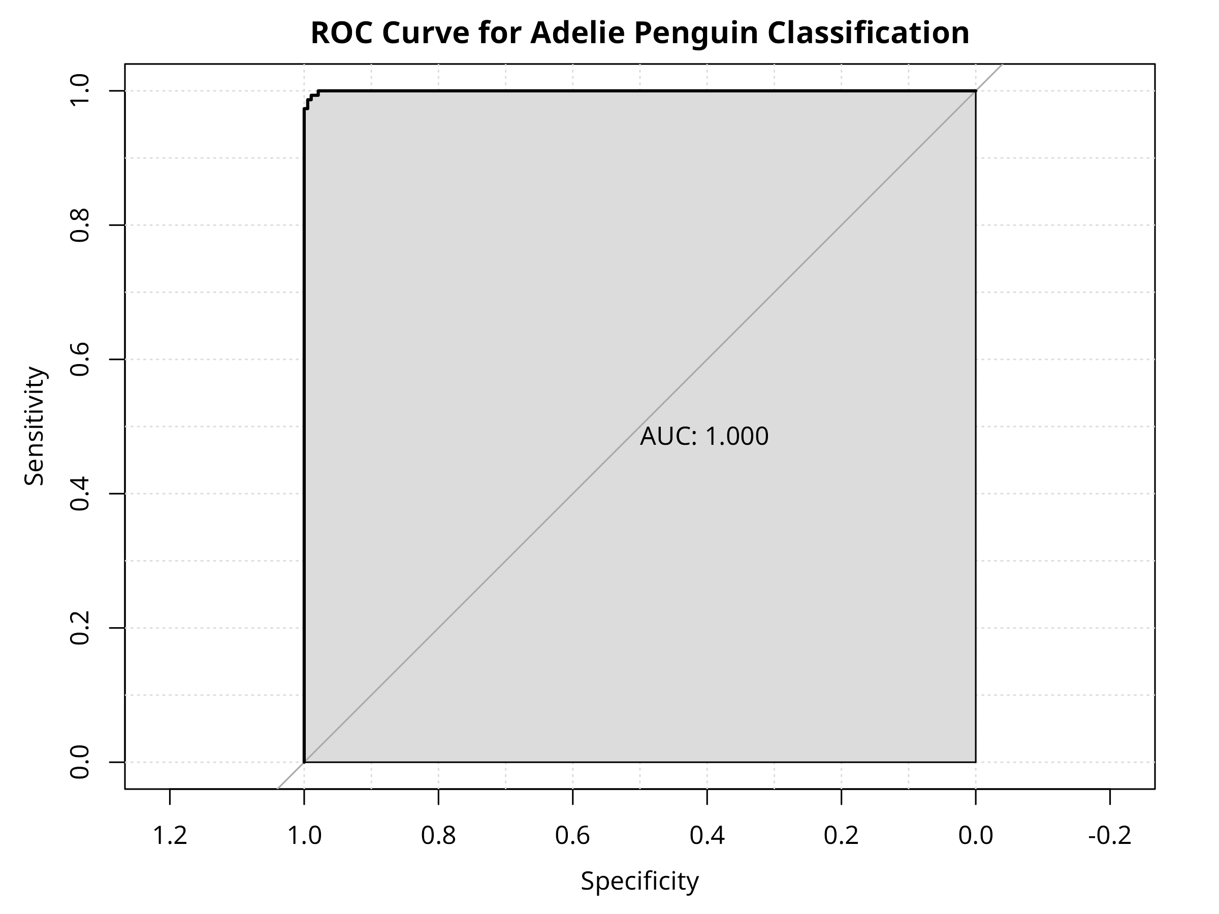
logistic_pred %>%
  roc_curve(truth = is_adelie, .pred_Adelie) %>%
  autoplot() +
  labs(title = "ROC Curve: Tidymodels Logistic Regression") +
  theme_minimal()

# Calculate AUC for use in next plot
auc_value <- logistic_pred %>%
  roc_auc(truth = is_adelie, .pred_Adelie) %>%
  pull(.estimate)

cat("Area Under the Curve (AUC):", round(auc_value, 3), "\n")
#> Area Under the Curve (AUC): 0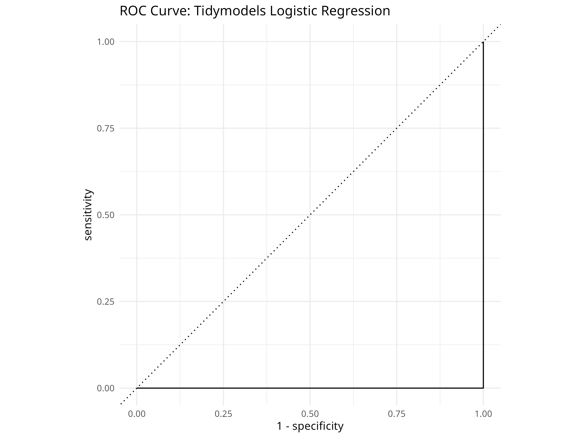
Code
ggplot(logistic_pred, aes(x = bill_depth_mm, y = body_mass_g,
                         color = .pred_Adelie, shape = is_adelie)) +
  geom_point(size = 3, alpha = 0.7) +
  scale_color_gradient2(low = "navy", mid = "white", high = "red",
                       midpoint = 0.5) +
  labs(
    title = "Predicted Probabilities: Adelie Classification",
    subtitle = paste0("AUC = ", round(auc_value, 3)),
    x = "Bill Depth (mm)",
    y = "Body Mass (g)",
    color = "P(Adelie)",
    shape = "Actual Species"
  ) +
  theme_minimal()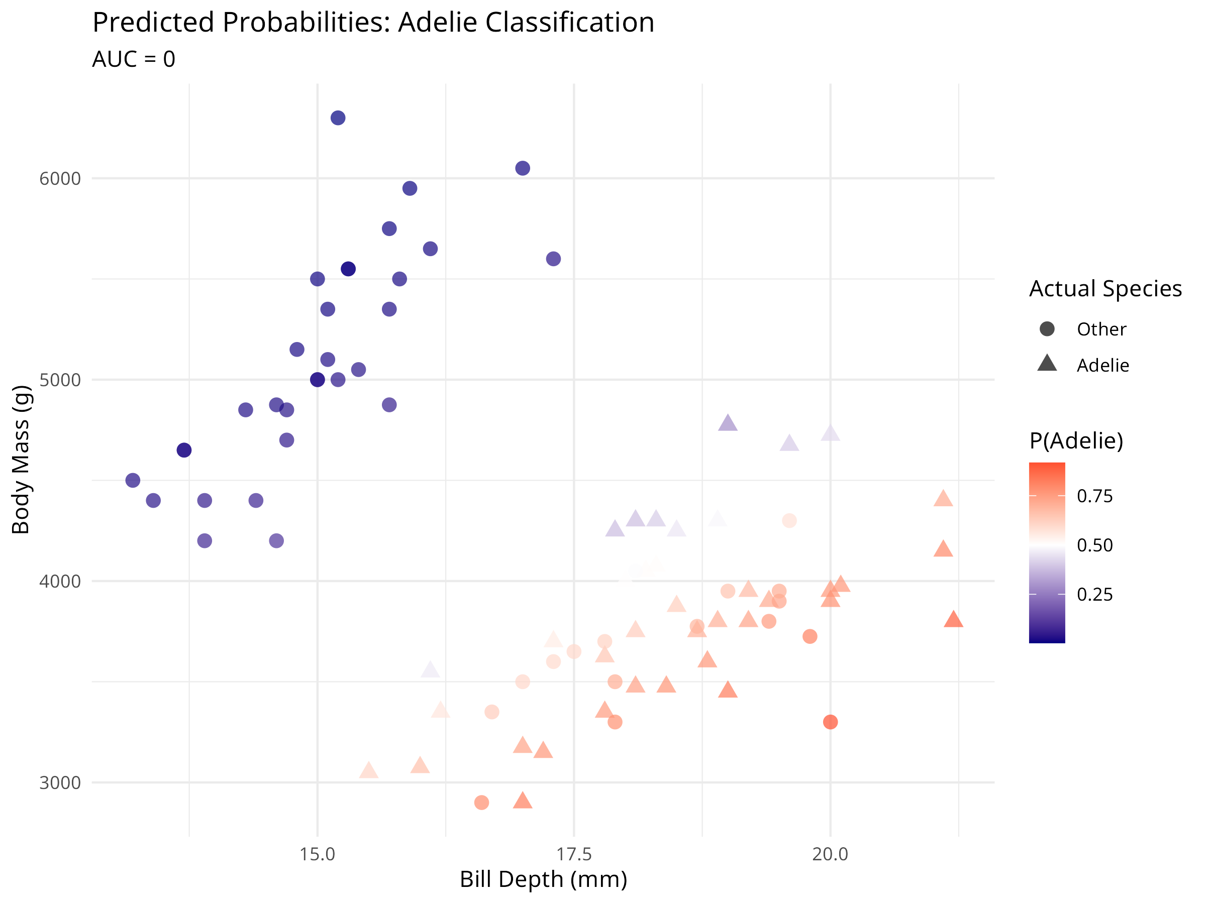
Tidymodels for Classification
The tidymodels classification workflow provides:
- Unified metrics: Automatic calculation of accuracy, ROC AUC, and other metrics
- Probability predictions: Easy access to class probabilities
- Visualization tools: Built-in plotting for confusion matrices and ROC curves
- Consistent interface: Same workflow structure as regression
8.8 Comparing Base R and Tidymodels Approaches
8.8.1 When to Use Each Approach
Base R (lm(), glm()) is ideal for: - Quick exploratory analyses - Simple models with few predictors - Teaching statistical concepts - When you need specific model diagnostics - Working with traditional statistical output
Tidymodels is ideal for: - Production modeling pipelines - Comparing multiple models - Complex preprocessing requirements - Cross-validation and resampling - Hyperparameter tuning - Consistent evaluation across models - Reproducible research workflows
8.8.2 Feature Comparison
| Feature | Base R | Tidymodels |
|---|---|---|
| Learning Curve | Moderate | Steeper initially |
| Consistency | Varies by package | Unified interface |
| Preprocessing | Manual | Automated with recipes |
| Cross-validation | Manual setup | Built-in support |
| Model Comparison | Manual | Streamlined |
| Hyperparameter Tuning | Package-specific | Unified with tune |
| Production Deployment | More complex | Workflow objects |
| Extensibility | High | Very high |
PROFESSIONAL TIP: Best of Both Worlds
Many practitioners use both approaches:
- Exploration: Use base R for quick model fitting and diagnostics
- Refinement: Transition to tidymodels for rigorous evaluation
- Production: Deploy tidymodels workflows for consistency
- Communication: Use base R output for traditional audiences, tidymodels for modern reports
8.9 Exercises
8.9.1 Base R Exercises
Fit a linear regression model predicting body mass from bill length and bill depth. Create a 3D visualization of this relationship using the
plotlypackage.Conduct multiple regression with interaction terms between predictors. How does adding interactions improve model performance?
Perform model selection using AIC to find the most parsimonious multiple regression model for the penguin data.
Create a multinomial logistic regression model to classify all three penguin species based on morphological traits.
Compare the performance of logistic regression with other classification methods (e.g., random forest, support vector machines) for species identification.
8.9.2 Tidymodels Exercises
Create a tidymodels workflow for predicting flipper length from body mass and bill measurements. Use 5-fold cross-validation to evaluate performance.
Build a recipe that includes polynomial features (e.g., squared terms) for bill length and bill depth. Compare this model’s performance to a linear model using cross-validation.
Use tidymodels to compare at least three different regression models (e.g., linear regression, random forest, support vector machine) for predicting body mass. Which performs best?
Create a classification workflow using tidymodels to predict all three penguin species. Calculate and compare precision, recall, and F1 scores for each species.
Implement a hyperparameter tuning workflow using
tune_grid()to optimize the number of trees and minimum node size for a random forest model predicting body mass.
8.9.3 Advanced Exercises
Split the penguin data by island, use one island as a test set, and evaluate how well models trained on other islands generalize. What does this tell you about geographical variation?
Create a nested cross-validation workflow: use an outer loop for model evaluation and an inner loop for hyperparameter tuning. Compare this to simple cross-validation.
-
Develop a complete modeling pipeline that includes:
- Data exploration and visualization
- Train/test split with stratification
- Recipe with appropriate preprocessing
- Multiple model specifications
- Cross-validation comparison
- Final model evaluation on test set
- Interpretation of results
Use tidymodels to implement a regularized regression (ridge or lasso) and compare it to ordinary least squares. How does regularization affect the coefficients?
Create an ensemble model that combines predictions from linear regression, random forest, and gradient boosting models. Does the ensemble outperform individual models?