Regression analysis is a powerful statistical tool for modeling relationships between variables. This chapter explores different types of regression models and their applications in natural sciences research.
8.2 Linear Regression
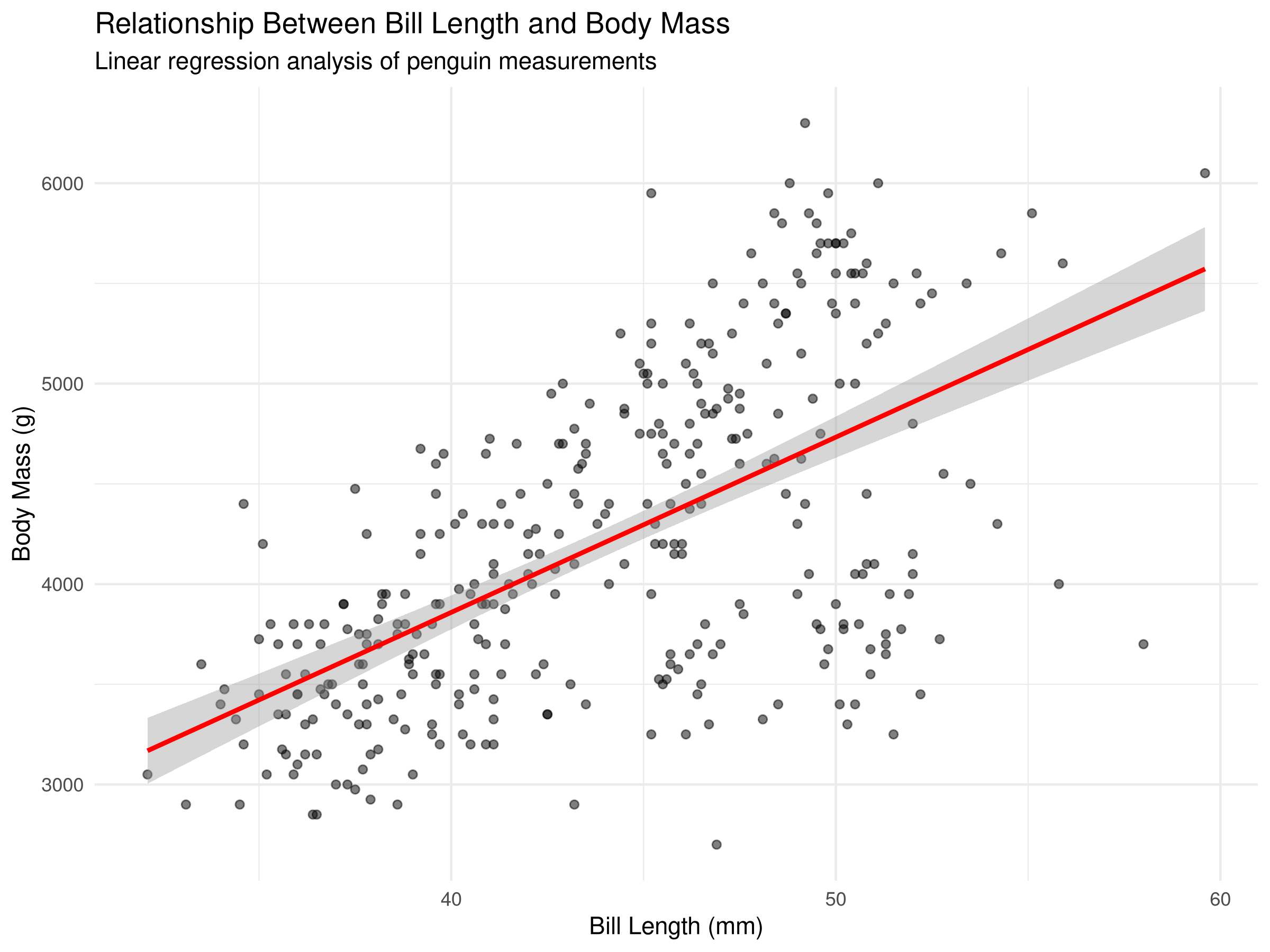
Linear regression models the relationship between a dependent variable and one or more independent variables:
Code
# Load required packageslibrary(tidyverse)library(ggplot2)library(broom) # For tidying model outputs# Load the Palmer penguins dataset (stored as climate_data.csv)penguins <-read_csv("../data/environmental/climate_data.csv")# Remove rows with missing values in the key variables we'll use for regressionpenguins <- penguins %>%filter(!is.na(bill_length_mm), !is.na(body_mass_g), !is.na(bill_depth_mm), !is.na(flipper_length_mm))# Create a linear regression modelmodel <-lm(body_mass_g ~ bill_length_mm, data = penguins)# Get model summarysummary(model)
Call:
lm(formula = body_mass_g ~ bill_length_mm, data = penguins)

Residuals:
     Min       1Q   Median       3Q      Max
-1762.08  -446.98    32.59   462.31  1636.86

Coefficients:
               Estimate Std. Error t value Pr(>|t|)
(Intercept)     362.307    283.345   1.279    0.202
bill_length_mm   87.415      6.402  13.654   <2e-16 ***
---
Signif. codes:  0 '***' 0.001 '**' 0.01 '*' 0.05 '.' 0.1 ' ' 1

Residual standard error: 645.4 on 340 degrees of freedom
Multiple R-squared:  0.3542,    Adjusted R-squared:  0.3523
F-statistic: 186.4 on 1 and 340 DF,  p-value: < 2.2e-16
Code
# Create a scatter plot with regression lineggplot(penguins, aes(x = bill_length_mm, y = body_mass_g)) +geom_point(alpha =0.5) +geom_smooth(method ="lm", color ="red") +labs(title ="Relationship Between Bill Length and Body Mass",subtitle ="Linear regression analysis of penguin measurements",x ="Bill Length (mm)",y ="Body Mass (g)" ) +theme_minimal()
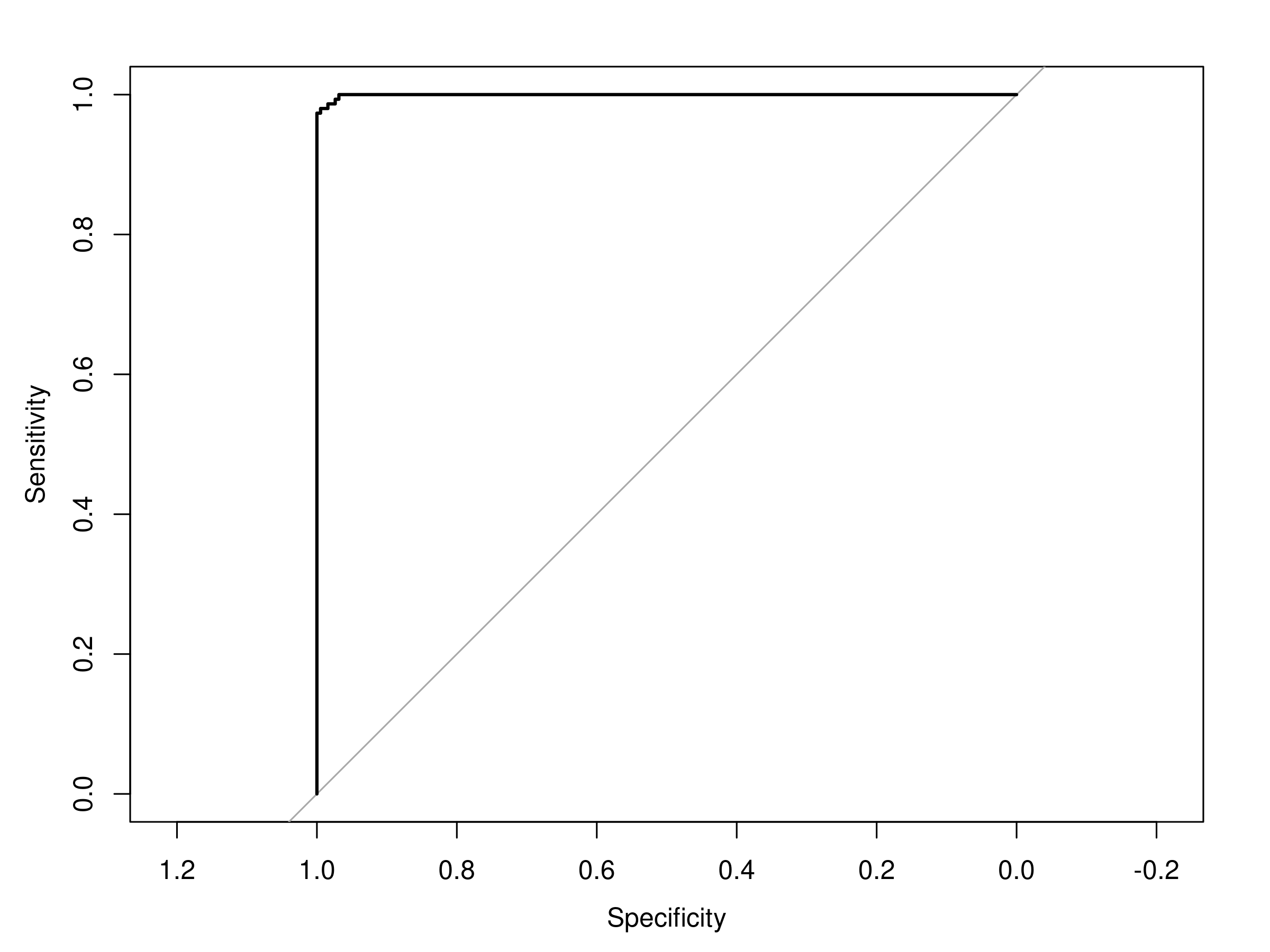
# Prepare data for logistic regression by creating a binary outcome# We'll predict whether a penguin is Adelie species or notpenguins_binary <- penguins %>%# Create a binary outcome variable (is_adelie)mutate(is_adelie =ifelse(species =="Adelie", 1, 0),# Convert to factor for better model interpretationis_adelie_factor =factor(is_adelie, levels =c(0, 1), labels =c("Other", "Adelie")))# Create logistic regression modellog_model <-glm(is_adelie ~ bill_length_mm + bill_depth_mm,family =binomial(link ="logit"),data = penguins_binary)# Get model summarysummary(log_model)
Call:
glm(formula = is_adelie ~ bill_length_mm + bill_depth_mm, family = binomial(link = "logit"),
    data = penguins_binary)

Coefficients:
               Estimate Std. Error z value Pr(>|z|)
(Intercept)     24.1355    13.5349   1.783  0.07455 .
bill_length_mm  -2.2103     0.6843  -3.230  0.00124 **
bill_depth_mm    3.9988     1.4833   2.696  0.00702 **
---
Signif. codes:  0 '***' 0.001 '**' 0.01 '*' 0.05 '.' 0.1 ' ' 1

(Dispersion parameter for binomial family taken to be 1)

    Null deviance: 469.424  on 341  degrees of freedom
Residual deviance:  18.708  on 339  degrees of freedom
AIC: 24.708

Number of Fisher Scoring iterations: 11
---prefer-html: true---# Regression Analysis## IntroductionRegression analysis is a powerful statistical tool for modeling relationships between variables. This chapter explores different types of regression models and their applications in natural sciences research.## Linear RegressionLinear regression models the relationship between a dependent variable and one or more independent variables:```{r}# Load required packageslibrary(tidyverse)library(ggplot2)library(broom) # For tidying model outputs# Load the Palmer penguins dataset (stored as climate_data.csv)penguins <-read_csv("../data/environmental/climate_data.csv")# Remove rows with missing values in the key variables we'll use for regressionpenguins <- penguins %>%filter(!is.na(bill_length_mm), !is.na(body_mass_g), !is.na(bill_depth_mm), !is.na(flipper_length_mm))# Create a linear regression modelmodel <-lm(body_mass_g ~ bill_length_mm, data = penguins)# Get model summarysummary(model)# Create a scatter plot with regression lineggplot(penguins, aes(x = bill_length_mm, y = body_mass_g)) +geom_point(alpha =0.5) +geom_smooth(method ="lm", color ="red") +labs(title ="Relationship Between Bill Length and Body Mass",subtitle ="Linear regression analysis of penguin measurements",x ="Bill Length (mm)",y ="Body Mass (g)" ) +theme_minimal()# Create diagnostic plotspar(mfrow =c(2, 2))plot(model)```::: {.callout-note}## Code ExplanationThis code demonstrates linear regression analysis:1. **Model Setup**: - Uses `lm()` for linear regression - Predicts body mass from bill length - Includes model diagnostics2. **Visualization**: - Creates scatter plot with regression line - Uses `geom_smooth()` for trend line - Adds appropriate labels3. **Diagnostics**: - Residual plots - Q-Q plot - Scale-location plot - Leverage plot:::::: {.callout-important}## Results InterpretationThe regression analysis reveals:1. **Model Fit**: - Strength of relationship (R²) - Statistical significance (p-value) - Direction of relationship2. **Assumptions**: - Linearity of relationship - Homogeneity of variance - Normality of residuals - Independence of observations3. **Practical Significance**: - Effect size - Biological relevance - Prediction accuracy:::::: {.callout-tip}## PROFESSIONAL TIP: Regression Analysis Best PracticesWhen conducting regression analysis:1. **Model Selection**: - Choose appropriate model type - Consider variable transformations - Check for multicollinearity - Evaluate model assumptions2. **Diagnostic Checks**: - Examine residual plots - Check for outliers - Verify normality - Assess leverage points3. **Reporting**: - Include model coefficients - Report confidence intervals - Provide effect sizes - Discuss limitations:::## Multiple RegressionMultiple regression extends linear regression to include multiple predictors:```{r}# Create multiple regression modelmulti_model <-lm(body_mass_g ~ bill_length_mm + bill_depth_mm + flipper_length_mm,data = penguins)# Get model summarysummary(multi_model)# Create diagnostic plotspar(mfrow =c(2, 2))plot(multi_model)```::: {.callout-note}## Code ExplanationThis code demonstrates multiple regression:1. **Model Structure**: - Multiple predictor variables - Additive effects - Model diagnostics2. **Analysis Components**: - Partial regression coefficients - Adjusted R² - F-test for overall fit3. **Diagnostic Tools**: - Multicollinearity checks - Residual analysis - Model comparison:::::: {.callout-important}## Results InterpretationThe multiple regression analysis shows:1. **Model Performance**: - Overall model fit - Individual predictor effects - Interaction effects2. **Variable Importance**: - Relative contribution of each predictor - Statistical significance - Practical significance3. **Model Diagnostics**: - Multicollinearity issues - Residual patterns - Model assumptions:::## Logistic RegressionLogistic regression models binary outcomes:```{r}# Prepare data for logistic regression by creating a binary outcome# We'll predict whether a penguin is Adelie species or notpenguins_binary <- penguins %>%# Create a binary outcome variable (is_adelie)mutate(is_adelie =ifelse(species =="Adelie", 1, 0),# Convert to factor for better model interpretationis_adelie_factor =factor(is_adelie, levels =c(0, 1), labels =c("Other", "Adelie")))# Create logistic regression modellog_model <-glm(is_adelie ~ bill_length_mm + bill_depth_mm,family =binomial(link ="logit"),data = penguins_binary)# Get model summarysummary(log_model)# Create ROC curvelibrary(pROC)roc_curve <-roc(penguins_binary$is_adelie, fitted(log_model))plot(roc_curve)```::: {.callout-note}## Code ExplanationThis code demonstrates logistic regression:1. **Model Setup**: - Creates a binary outcome variable (is_adelie) - Uses logit link function - Includes multiple predictors2. **Analysis Components**: - Odds ratios - Classification accuracy - ROC curve analysis3. **Visualization**: - ROC curve - Classification plots - Diagnostic plots:::::: {.callout-important}## Results InterpretationThe logistic regression analysis reveals:1. **Classification Performance**: - Model accuracy - Sensitivity and specificity - ROC curve characteristics2. **Predictor Effects**: - Odds ratios - Confidence intervals - Statistical significance3. **Model Diagnostics**: - Classification errors - Residual patterns - Model fit:::## SummaryIn this chapter, we've explored different types of regression analysis:- Linear regression for continuous outcomes- Multiple regression for multiple predictors- Logistic regression for binary outcomesEach type has specific applications and assumptions that must be considered when analyzing natural science data.## Exercises1. Fit a linear regression model predicting body mass from bill length and bill depth.2. Create diagnostic plots for your model and interpret them.3. Compare the performance of different model specifications.4. Conduct a logistic regression analysis for species classification.5. Create and interpret ROC curves for your logistic regression model.